CURVE FITTING

• CURVE FITTING:

• AIM:

The main aim of the project is to write the program to fit the linear and cubic polynomial for specific heat(cp) data and temperature.

• OBJECTIVE:

Curve fitting is a process of constructing a curve or mathematical model to a given certain data points, possibly subjected to constraints. Curve fitting can involve either interpolation,where an exact fit to the data is required or smoothing in which smooth function is constructed that approximately fits the data.

• POLYNOMIAL FUNCTION:

First degree polynomial equation / Linear equation:

Equation :y=ax+b">y=ax+by=ax+b

Second degree polynomial equation/Quadratic equation:

Equation: y=ax2+bx+c">y=ax2+bx+cy=ax2+bx+c

Third degree polynomial equation/cubic equation:

Equation: ax3+bx2+cx+d">ax3+bx2+cx+dax3+bx2+cx+d

• EXPLANITION:

1. The file containing the data is extracted by giving a command called 'load' .
2. As we know that the first column of data is temperature and second column is cp ,indicate same in MATLAB
3. polyfit command computes a least square polynomial for a given set of data,and it generates the coefficient of the polynomial which is used to construct the curve to fit the data.
4. polyval command evaluates the coefficient and generate a curve using the data based on the coefficient obtained from polyfit command.
5. plot the data and compare with the original set of data by using the plot command to get the linear and cubic curve fitting.
6. legend is provided to the plot to diffentiate between the original and predicted values.

• CODING FOR LINEAR EQUATION:

clear all
close all
clc

%program to fit a linear curve y = ax+b

cp_data = load('data');
temp = cp_data(:,1);
cp = cp_data(:,2);

%To find the coefficient

co_eff = polyfit(temp,cp,1);
 
%To calculate cp using co_eff

pre_cp = polyval(co_eff,temp);

%ploting
%original dataset
plot(temp,cp,'color','r');
hold on
plot(temp,pre_cp,'color','b');
hold off
xlabel('temperature[k]')
ylabel('specific heat[kj/k-mol k]')

• PLOT:

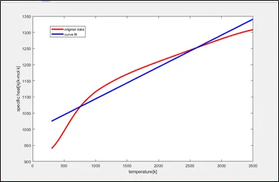
It can be observed that their is large error in the curve fit and hence curve doesn't fit perfectly.

• TOOLBOX:

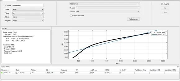
If we consider R square as a tool to comapre the goodness of fit ,then its value is 0.9249.Hence it is not a good fit.

• SOLUTION:

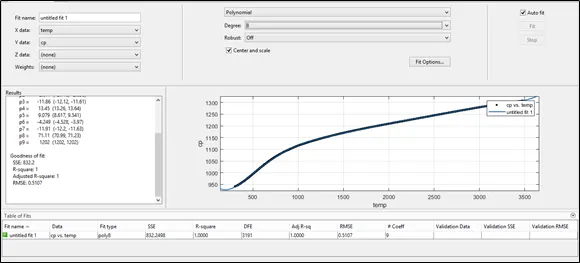
To get a perfect fit/increase the goodness of fit ,we need to get the value R-square equals to 1, this can be obtained by increasing the order to 8 and enabling the center and scaling.

1. Centring a variable is subtracting the mean of the variable from each data point so that the new variable's mean is 0.
2. Scaling a variable is multiplying each data point by a constant in order to alter the range of the data.
3. Best fit means the difference between the original dataset and curve fit data set values by model equation are minimized.
4. Perfect fit means curve goes through every single data set and R-SQUARE value is equal to 1

• CODING FOR CUBIC POLYNOMIAL:

clear all
close all
clc

%program to fit a cubic curve y = ax^3+bx^2+cx+d

cp_data = load('data');
temp = cp_data(:,1);
cp = cp_data(:,2);

%To find the coefficient

co_eff = polyfit(temp,cp,3);
 
%To calculate cp using co_eff

pre_cp = polyval(co_eff,temp);

%ploting
%original dataset
plot(temp,cp,'color','r','linewidth',3);
hold on
plot(temp,pre_cp,'color','b','linewidth',3);
hold off
xlabel('temperature[k]')
ylabel('specific heat[kj/k-mol k]')

• PLOT:

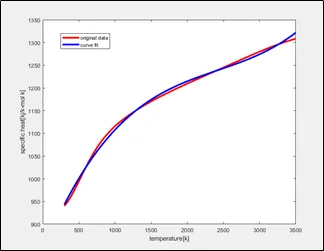
It can be observed that their is a small error in the curve fit and hence it doesn't fit perfectly.

• TOOLBOX:

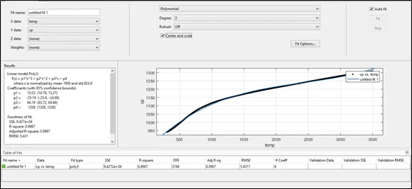
If we consider the R-square as a tool to compare the goodness of fit, it's value is 0.9967 which is very near to 1 hence it is a good fit.

• SOLUTION:

To increase the goodness of fit of cubic polynomial we can use splitting the data technique as shown below.

clear all
close all
clc

%input
cp_data = load('data');
temp = cp_data(:,1);
cp = cp_data(:,2);

%splitting the data

co_eff1 = polyfit(temp(1:1600),cp(1:1600),3);
co_eff2 = polyfit(temp(1600:3200),cp(1600:3200),3);

%To calculate cp using coeff1 &coeff2

pre_cp1 = polyval(co_eff1,temp(1:1600));
pre_cp2 = polyval(co_eff2,temp(1600:3200));

%plotting

plot(temp,cp,'linewidth',3,'color','r');
hold on
plot(temp(1:1600),pre_cp1,'linewidth',1,'color','b');
plot(temp(1600:3200),pre_cp2,'linewidth',1,'color','y');
hold off
xlabel('temperature[k]');
ylabel('specific heat[kj/k-mol k]');

• PLOT:

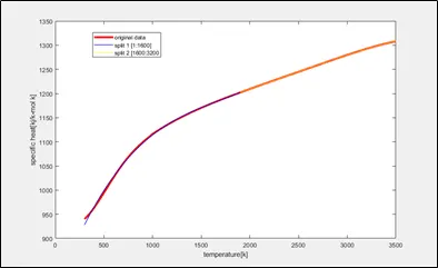
We can observe that by splitting the data we get better fit than the earlier cubic fit.

• REFERENCES:

1. https://en.wikipedia.org/wiki/curve_fitting
2. https://projects.skill-lync.com/projects/Curve-Fitting-and-criterion-to-choose-best-fit-41860