Week 3 - Solving second order ODEs

• SIMULATION OF SIMPLE PENDULUM:

• AIM:

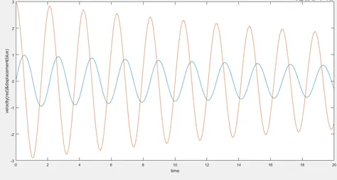
The main aim the project is to simulate the motion of simple pendulum using the MATLAB code and to plot the velocity and displacement variation with respect to the time.

• OBJECTIVE:

A simple pendulum consist of mass (m) attached by a string or rod of length(l) . When it is displaced to an initial angle and released, the pendulum will swingh back and forth with periodic motion.The figure shows the simple pendulum

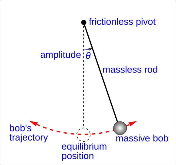
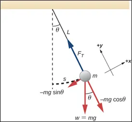
FIG: SIMPLE PENDULUM FIG: FREE BODY DIAGRAM OFSIMPLE

PENDULUM

• GOVERNING EQUATION:

This equation represents the equation of motion of simple pendulum with damping.

`(d^2theta)/dt+b/m*(d theta)/dt+g/l * sin(theta) = 0`

Breaking the governing equation;

say `theta = theta1` .............(1) where b = damping coefficient

upon diffentiation w.r.t t we get, g = acceleration due to gravity in m/s^2

`(d theta)/dt = (d theta1)/dt = theta2`..........(2) l = length of rod in m

again upon diffentiation m = mass of bob in kg

`(d^2 theta)/dt^2 =(d^2 theta1)/dt^2 = (d theta2)/dt` ................(3)

from (2) and (3) we get

`(d theta1)/dt = theta2`

and `(d theta2)/dt = -(b/m)*theta2 - (g/l)*sin(theta1)`

• EXPLANATION:

1. Bring all the input values like damping coefficient , acceleration due to gravity ,length of the rod ,mass of the bob.
2. Enter the initial condition angular displacement and angular velocity and time span using linspace command.
3. use ode45 solver to solve the differential function but before that we have to call the ode function using function command.
4. plot the variation of angular displacement and angular velocity with respect to time using plotting command.
5. For loop is initiated and coordinates of the rod is given and the bob is created by using the commands like plot and the size of bob is given by markersize string.
6. videowriter command is used to create the blank avi file and writevideo command will collect all the frames and create the simulation of the simple pendulum.

• PROGRAM:

clear all
close all
clc

%inputs

b = 0.05;
l = 1;
m = 1;
g = 9.81;

%initial condition

theta_0 = [0;3];

t_span = linspace(0,20,200);

%ODE SOLVER

[t,result] = ode45(@(t,theta) ode_func(t,theta,b,g,l,m),t_span,theta_0);

%plotting

figure(1)
plot(t,result(:,1));
hold on
plot(t,result(:,2));
xlabel('time')
ylabel('velocity(red)&displacement(blue)')

ct = 1
theta = result(:,1)

for i = 1:length(theta)
    THETA = theta(i);

x0 = 0;
y0 = 0;
 
x1 = l*sin(THETA);
y1 = -l*cos(THETA);

figure(2)
plot([x0 x1],[y0 y1],'linewidth',4)
hold on 
plot(x1,y1,'-o','MarkerSize',10,'color','r','MarkerFaceColor','b')
hold off
axis([-2 2 -2 2]);
M(ct) = getframe(gcf)
ct = ct + 1
pause(0.03)

end

movie(M)
video_file = VideoWriter('Pendulum.avi','Uncompressed AVI');
open(video_file)
writeVideo(video_file,M)
close(video_file)

The following function code has been called in the above MATLAB programme.

function [dtheta_dt] = ode_func(t,theta,b,g,l,m)

theta1 = theta(1);
theta2 = theta(2);
dtheta1_dt = theta2;
dtheta2_dt = -(b/m)*theta2-(g/l)*sin(theta1);
dtheta_dt = [dtheta1_dt;dtheta2_dt];
end

• CONCLUSION:

The simulation of simple pendulum is obtained and the graph has been plotted

• PLOT:

• LINK:

https://youtu.be/coBwV7uJ-nA