Simulation of a backward facing step in OpenFOAM

Week 8 Report

• Aim: To simulate an incompressible-laminar-viscous flow through the backward facing step geometry using OpenFoam.
  
  
  
  
• Theoretical Introduction:
  
  OpenFOAM (for "Open-source Field Operation And Manipulation") is a C++ toolbox for the development of customized numerical solvers, and pre-/post-processing utilities for the solution of continuum mechanics problems, most prominently including computational fluid dynamics (CFD).
  
  
  

  OpenFOAM simulations are configured by several plain text input files located across the following three directories:

  • system:
    • controlDict
    • fvSchemes
    • fvSolution
    • fvOptions (optional)
    • (other dictionaries (configuration files in OpenFOAM))
      
      
  • constant
    • polyMesh/other dictionaries)
      
      
  • 0/ (or another initial time directory)
    • field files

  Additional directories can be generated, depending on user selections. These may include:

(result time directories): field predictions as a function of iteration count or time

There are certain Advantages and Diadvantages of using OpenFoam, some of which are:

Advantages:

• Friendly syntax for partial differential equations
• Fully documented source code
• Unstructured polyhedral grid capabilities
• Automatic parallelization of applications written using OpenFOAM high-level syntax
• Wide range of applications and models ready to use
• Commercial support and training provided by the developers
• No license costs

Disadvantages:

• The development community suffers from fragmentation, giving rise to numerous forked projects.
• Absence of an integrated graphical user interface (stand-alone open-source and proprietary options are available)
• The Programmer's guide does not provide sufficient details, making the progress slow if you need to write new applications or add functionality

• Case-setup:
  
  1. To begin to perform the case-setup, we must open the terminal and then open the Incompressible folder in the Tutorials present in the OpenFoam Folder. To access the incompressible folder, we must type in the command of "tut" in the terminal.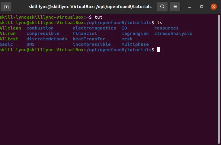
  
  
  
  Tutorials in OpenFoam
  
  
  2.Then inside the Incompressible Folder, open the Ico-Foam folder. Then next step would be to copy the cavity folder in the Run folder of OpenFoam. To copy this folder, we can use the command of "cp -r cavity/ destination_folder/ name of the folder after copying". So in our case, the code will be as follows:
  
  cp -r cavity /$FOAM_RUN/cavity_week8
  
  -r is a command telling the software to copy all the folders recursively.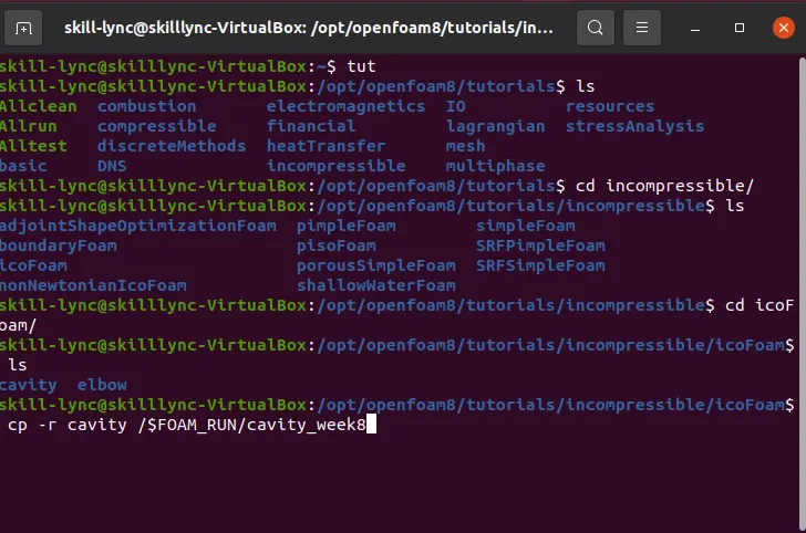
  
  
  
  Copying Files to a destination location
  
  
  After the copy was done, we are able to see the Folder copied in the run file: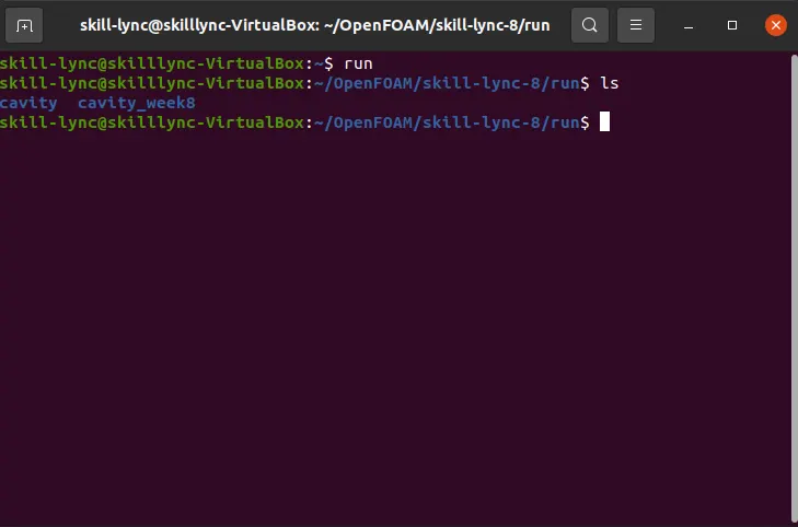
  
  
  
  Copied Files
  
  
  3. After the cavity folder is copied in the Run folder, then we must change certain properties of this folder to match the case set up that we desire. To access the run folder, we must simply use the command "run" and then edit the BlockMeshDict folder. This BlockMeshDict file is in the system folder in the main cavity folder. Inside this folder, we see the three main basic files, that will help us perform our simulation as per our needs. The '0" folder is the one where we insert all the Initial Conditions. In the constant folder, we will have the Polymesh and the Transport Properties folder as well. This transport properties folder will help us define the fluid flow properties for the simulation.
  Inside the system folder, we will have other folders that will help us define properties and simulation related criterias.
  To edit this folder, we need to use the command of "gedit" and then the folder name. This opens an editable file where in we can set up the case as and what we require.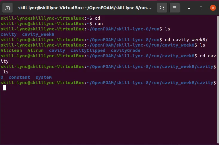
  
  
  
  Three files in the copied Folder
  
  
  4. In our case, we have set up 5 blocks to define the shape of the backward facing step on the geometry according to the geometry required in the question. These blocks are defined using certain co-ordinates. These co-ordinates are then used to define the local co-ordinate system that the block is supposed to use.
  The total number of co-ordinate points in the entire geometry are 21 and they are defined according to the number of blocks and the dimensions of the geometry. These co-ordinate points are then defined for all the three global axes according to the dimensions and the scaling factor that we have used for the set-up.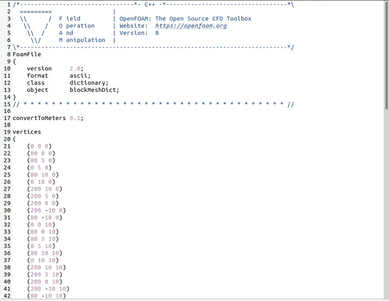
  
  
  
  Vertices Defined
  
  
  5. After we define the vertices of all the blocks, the next step is to define the blocks themselves. To do this, we use the blocks command and then define the blocks in a specific orientation. The placing of the vertices to define the blocks will then be used to define the local-co-ordinate axes. So the line connecting the first point and the second vertex will be used as the local x-axis for the block. The line connecting the second and the third point will be used as the local y-axis, and the Axis that is perpendicular to these two axes is used as the local z-axis for the block.
  Like, this we have to define the local co-ordinate system for all the blocks. Another factor that we must consider while forming the blocks is the factor if points in the x,y, z axis. Also, we must mention the grading for the mesh on the blocks.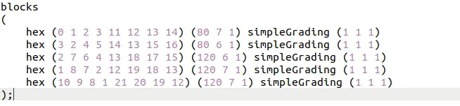
  
  
  
  Blocks Defined
  
  
  6. After defining the blocks we have almost completed the set-up for this backward facing step geometry. One of the last few steps is the step of assigning the Boundary conditions for the geometry. It is according to the Boundary Conditions, that the problem will be solved. We must assign the type of boundary conditions and the vertices for the same. While assigning the vertices, we must take care of the normal of the block that we are defining. The normal of the block must be facing outward and away from the geometry. We must then divide our boundary conditions on the basis of type of the boundary condition and even to ease out out understanding of the problem.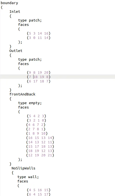
  
  
  
  
  Boundary Conditions(1)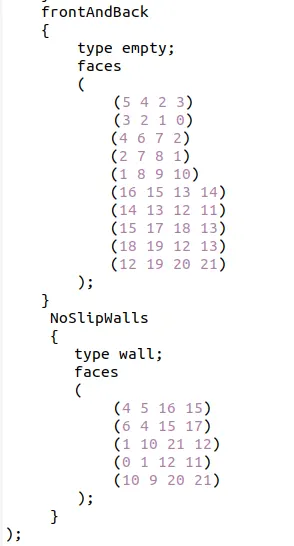
  
  
  
  
  Boundary Conditions(2)
  
  
  
  7. This is how we define the Boundary Conditions and the Blocks where we further define the mesh and the grading on that mesh. After this, we must run the blockMesh command in the run file. To view the mesh, we simply need to use the ParaView tab. To open this Paraview tab, we must use the "ParaFoam" command. The mesh will look something as the following.
  We must study this geometry when it is having a simple Grading of 1 and when it is having a grading of 0.2. Grading can be defined as the ratio of the length of the end cell to the length of the starting cell. So, when the grading is 0.2, it means that the length of the end cell is 5 times the length of the starting cell. Since the length is smaller for the starting cell, the mesh is finer at the location and the mesh is coarser at the end.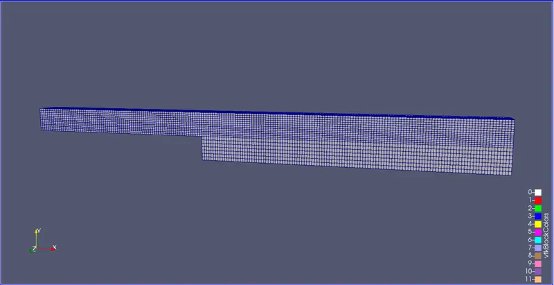
  
  
  
  Mesh with Grading factor = 1
  
  
  8. The last step is to run the "Ico-Foam" Solver in the run folder of the Software. To run the solver, we must simply give the command of "ico-Foam" in the run folder. This command runs the set-up according to Solver that we have selected. After running, we must then post-process the results in the Post-processing tool known as paraView. To access this tool, we simply give the command of "paraFoam" and then study the required output at different time-steps.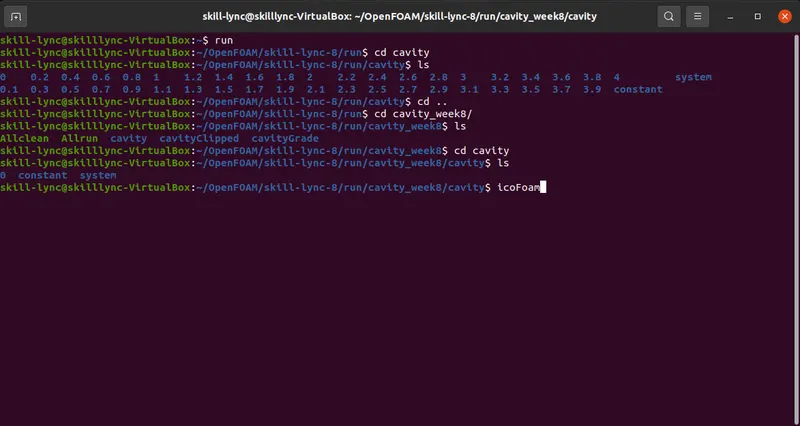
  
  
  
  Running the icoFoam Solver
  
  
  
  9. The final output that was required, is to measure the velocity profile at 0.085 m from the inlet of the geometry. To do this, we must use the option of Plot over line and then plot the line at the required location and then we must select the quantities that we wish to plot in the graph. To edit the graph, we can add the x-axis and the y-axis labels and also add the title of the graph.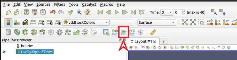
  
  
  
  
  Plot-over Line command
  
  After selecting the option, we must then draw the line using the x,y,z co-ordinates of the desired location as shown below: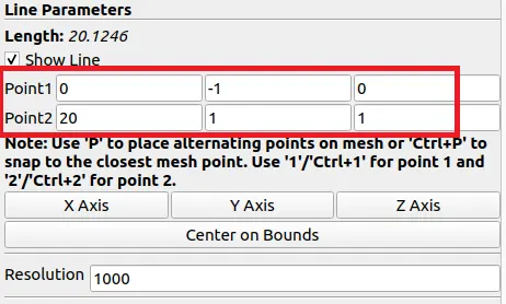
  
  
  
  Points to define the line across the Geometry.
  
  
  Here, we can define the co-ordinates of the two points to join them with a line.
  
  Next, we have to select the properties that we must measure across the line: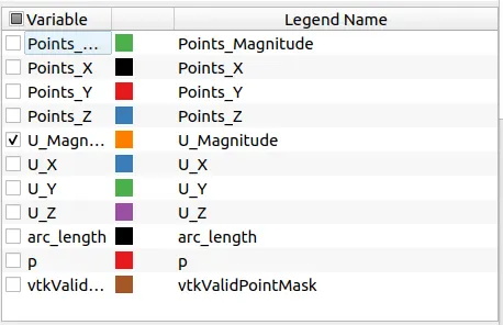
  
  
  
  Measuring the required Properties
  
  
  
  
  
  
  
• Results:
  
  1. The Plots for the Velocity measured for two different gradings of the mesh:
  
  Grading = 1.0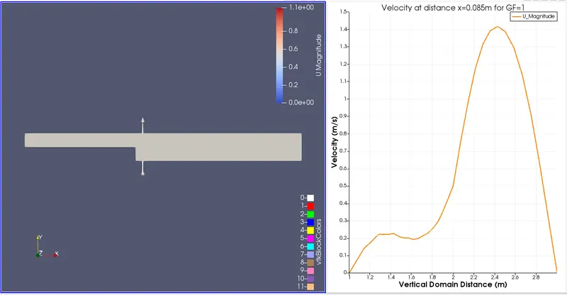
  
  
  
  
  Grading = 0.2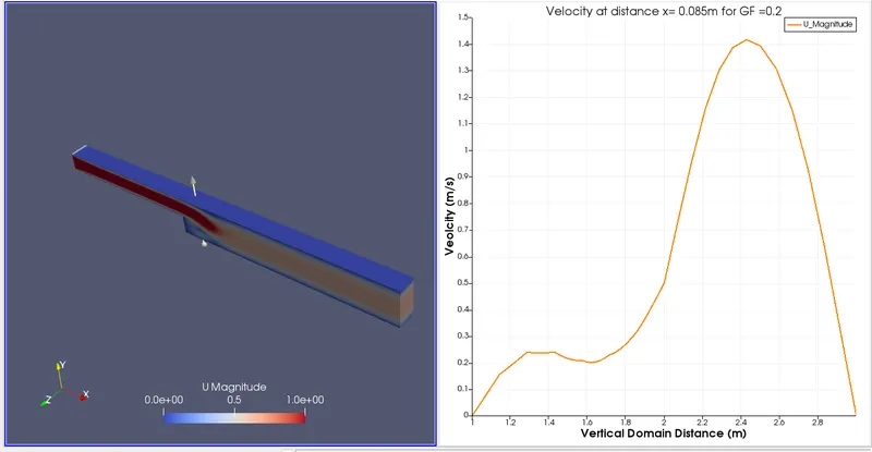
  
  
  
  As we can see from the above two plots, we can conclude that the results have not varied for when we change the grading from 1.0 to 0.2 for the mesh. The reason is that the mesh does not affect the physics or the conditions of the problem. Changing the grading of the mesh can be done for simply changing the area of focus of study in the problem. For example, if the Mesh is much more finer near the Boundary, it means that the accuracy of the simulation is higher near to the boundary. We can change the mesh grading according to our need and focus of study.
  Grading/Growth Factor is essential for the process of meshing as we can change or increase the accuracy of the simulation to a certain location in the geometry and change our focus to that particular point.
  
  
  
  
  
  
  
  
  
  
  
• Conclusion: In conclusion, I would like to state that this challenge helped me gain a much better understanding of OpenFoam and how to make and simulate simple Geometires in it.
•