Week 8 - Simulation of a backward facing step in OpenFOAM

WEEK 8 - SIMULATION OF A BACKWARD FACING STEP IN OpenFOAM

AIM:

• To simulate an incompressible-laminar-viscous flow through the backward facing step geometry.
• To perform a transient simulation.
• To measure the velocity profile at 0.085 m from the inlet of the geometry for both case studies and compare. You can use the plot over line tool for this.
• To explain why Grading/Growth factor is essential for meshing.
• To perform 2 case studies as described below and compare the results.

  Case - 1 - Simulate the flow without using any grading factor (i.e., GF = 1)

  Case - 2 - Simulate the flow with grading factor of 0.2. The cells should be finer near the walls (includig the step wall)

DESCRIPTION:

OPENFOAM:

OpenFOAM (for "Open-source Field Operation And Manipulation") is a C++ toolbox for the development of customized numerical solvers and pre-/post-processing utilities for the solution of continuum mechanics problems, most prominently including computational fluid dynamics (CFD).

There are three main variants of OpenFOAM software that are released as free and open-source software under the GNU GENEARAL PUBLIC LICENSE Version 3.

1. OpenFOAM variant by OpenCFD Ltd.
2. FOAM-Extend variant by Wikki Ltd.
3. OpenFOAM Foundation Inc.

OPENFOAM STRUCTURE:

Software structure:

The OpenFOAM layout consists of two main directories:

• OpenFOAM-: OpenFOAM libraries whose directory layout is shown in the side-figure
• ThirdParty: A set of third-party libraries.

Simulation structure

OpenFOAM simulations are configured by several plain text input files located across the following three directories:

• system/:
  • controlDict
  • fvSchemes
  • fvSolution
  • fvOptions (optional)
  • (other dictionaries (configuration files in OpenFOAM))
• constant
  • polyMesh/
  • (other dictionaries)
• 0/ (or another initial time directory)
  • (field files)

Additional directories can be generated, depending on user selections. These may include:

• (result time directories): field predictions as a function of iteration count or time
• postProcessing/: data typically generated by function objects data conversion, e.g. VTK

GIVEN CONDITIONS:

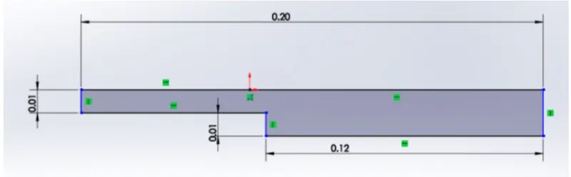
This is the 2 - d diaram of the structure which is given in the question.

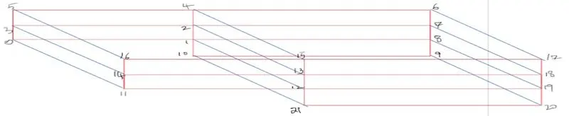
This is the 3 - d diagram of structure wich is divided into five blocks to make the simulation good.

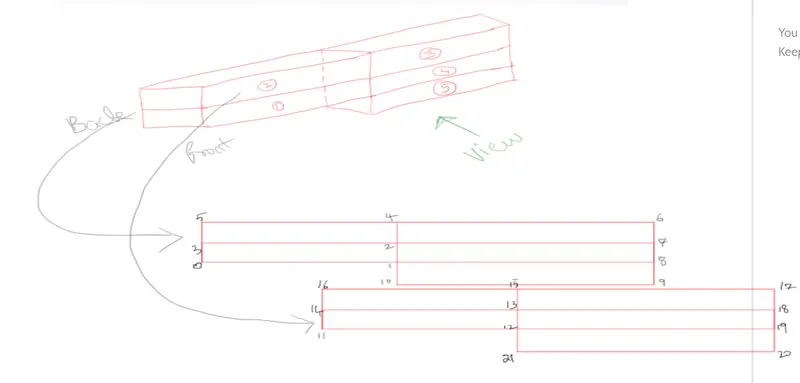
This diagram helps us to see all the direction views with numbered blocks

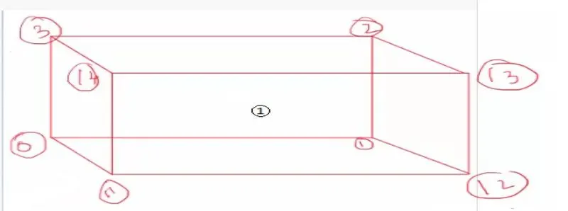
This is the 3 - D diagram of the block number one

STEP BY STEP PROCEDURE:

STEP-1:

First, we need to install the visual box and then we need to install the ubuntu in our system.

STEP-2:

we need to install the openFOAM software in ubuntu

STEP-3:

Now we need to open the terminal from the ubuntu desktop.

STEP-4:

The terminal is the command window where we can access to the folders, parafoam.

STEP-5:

cd - is the keyword which resembles "current directory"

ls - is the keyword which resembles "list" and it is used to list down the elements inside the folder.

In the terminal, we need to open the tutorials by using the command "cd $FOAM_TUTORIALS"

and followed by is explained in the picture

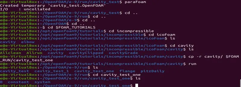
• From the picture we can see that after opening the tutorials we need to choose "cd incompressible", then "cd icoFoam"
• This icoFoam is used to calculate incompressible Navier Stoke's equation.
• From there we need to open the "cd cavity" and we need to copy this file in our directory so that we can run this by using the command "cp -r cavity/$FOAM_RUN/cavity_test".
• This cavity_test is the folder where we are going to save what we require.
• we will be having "0", "constant", "system" after listing down.

STEP-6:

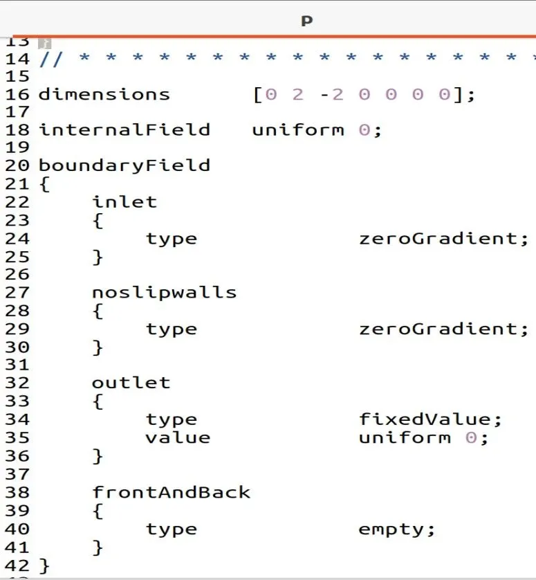
• By selecting "0" we will get two options one is "P" which is pressure and the other is "U", which is velocity. This has to be opened and it as to be edited according to our requirements and this can be done by using the command "gedit p" and "gedit u". "gedit" is a command which is used to open it because it is editable file.
• Now we need to give the values according to our requirements which is shown below.

STEP-7:

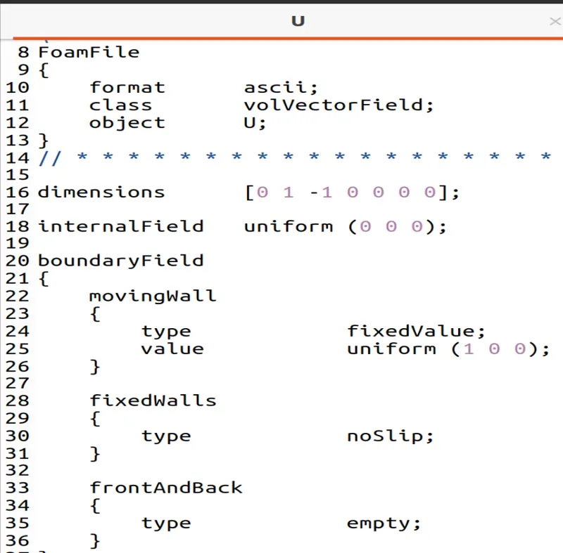
Similarly, we need to do for velocity file.

STEP-8:

• Now we need to open "system" and there we need to select "blockMeshDict" and we need to edit the following:
• "hex" is the keyword which resembles the type of mesh.
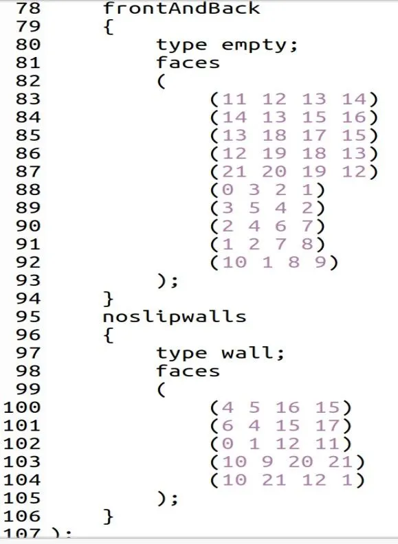
• Next to that is numbered faces of five geometry blocks.
• Next to that is to define number of cells along x, y and z axis.
• "simpleGrading" is the keyword which resembles grading factor and here in this case - 1 is "1".
• This part is to generate mesh.

STEP_9:

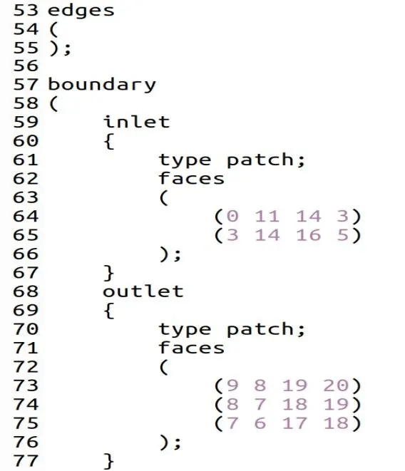
• In the blockMeshDict itself, we need to give the following details.
• We need to give boundary conditions such as "inlet", "outlet", "frontandback" and "noslipwalls"

STEP-10:

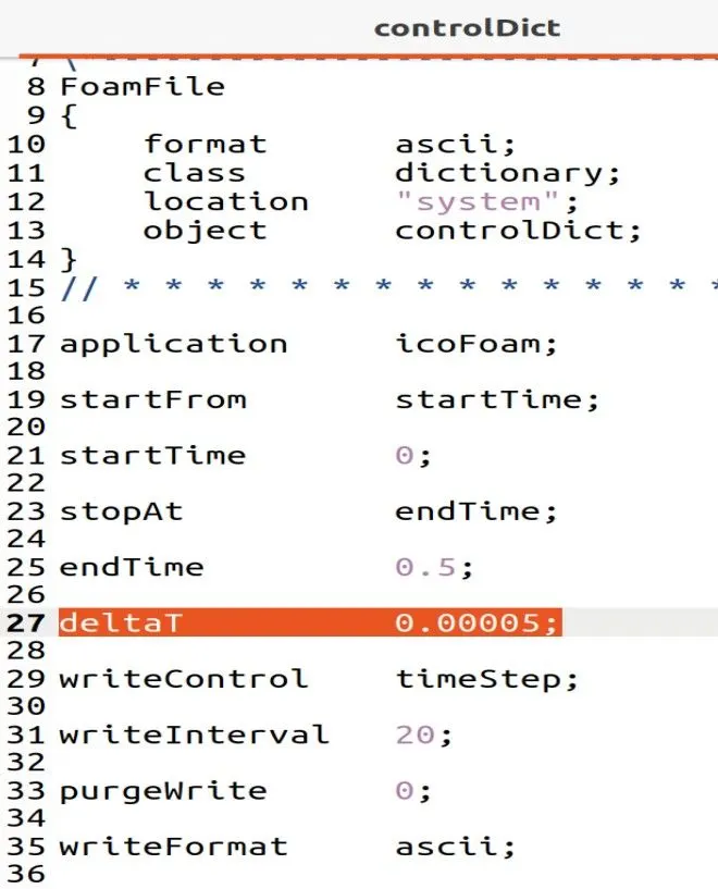
• Now we need to open "system" and there we need to select "controlDict" and we need to edit the following:
• We need to make sure that CFL number should be less than "0.5"

STEP-11:

• For case - 2, we need to keep all the settings constant an the only thing has to be changed is grading factor.

STEP-12:

After completing all these settings, we need to save the things what we have done by pressing the "save" button which is on the right side top or "ctrl + s"

STEP-13:

Now we need to go back to the terminal and we need to give the command "blockMesh"

STEP-14:

Now the mesh generation is done. Then we need to solve the problem by using "icoFoam" solver.

STEP-15:

To view the simulation or simulated results, we need to open paraview and to that we need to give the command "paraFoam"

RESULTS AND OUTPUT:

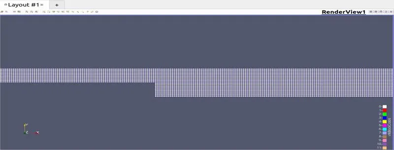
After opening the paraview, we can able to see the meshed structure.

CASE-1: meshed structure with GF =1.

CASE-2: meshed structure with GF 0.2 and 5

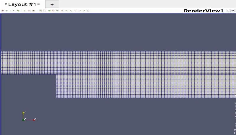
• By comparing to two cases, we can say that case 1 is uniform in structure with equal length of cells.
• The case 2 is different from case 1, because grading factor is introduced, at some parts cells are refined, the mesh looks congested at some parts of the structure.

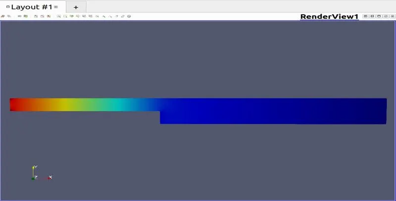
CASE-1: Pressure layout for GF = 1

CASE-2: Pressure layout for meshed structure with GF 0.2 and 5

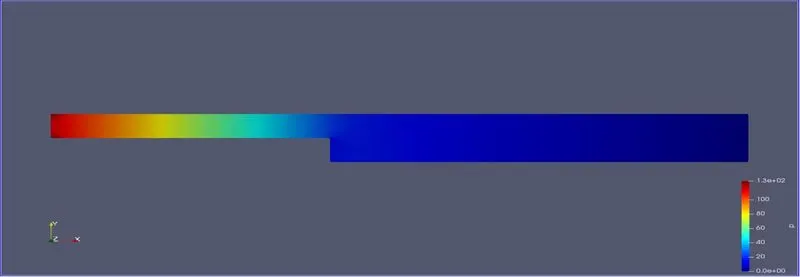
From the above two plots we can say that there is no much deviation.

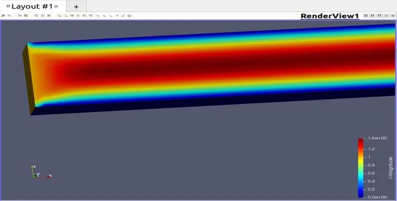
CASE-1: velocity layout for GF = 1

CASE-2: velocity layout for GF 0.2 and 5

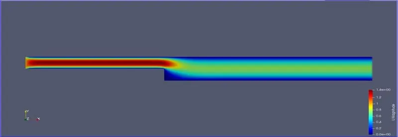
By comapring the above two plots, we can say that there is no much difference, but to examine the small difference, we need to use some other command to capture the small change in flow physics and i have explained in the last.

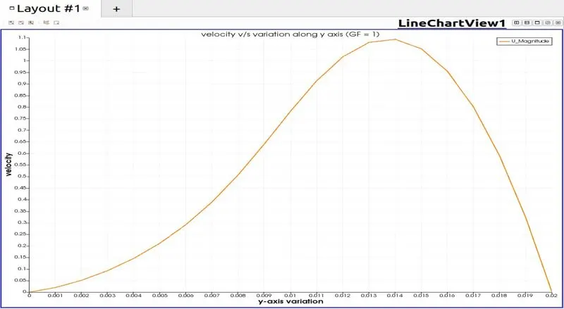
CASE-1: velocity plot for GF = 1

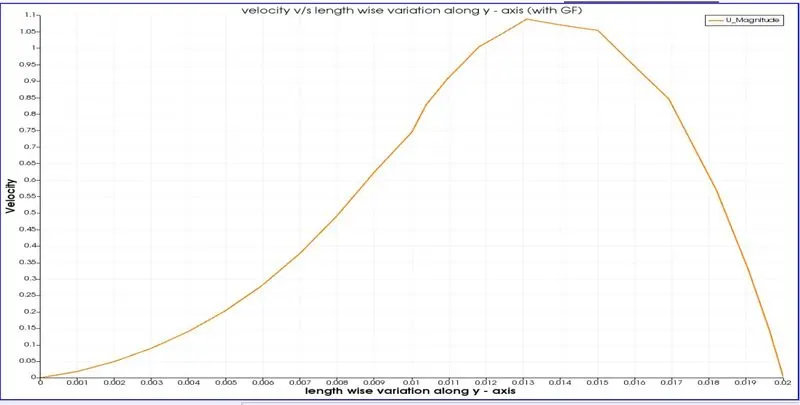
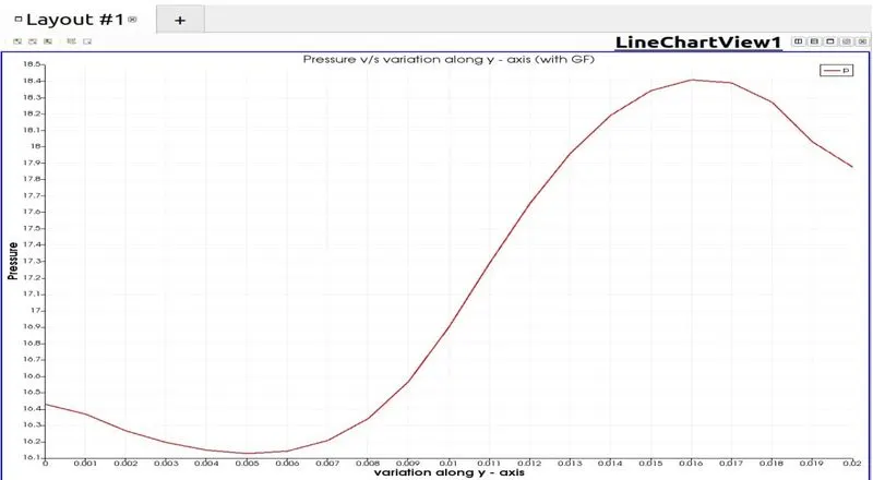
This plots are done by using the "plot over line" option which is available in the paraview and we need to select the fields what we want like pressure, density, temperature and velocity etc..

CASE-2: velocity plot for GF 0.2 and 5

CASE-1: Pressure plot for GF = 1

CASE-2: pressure plot for GF 0.2 and 5

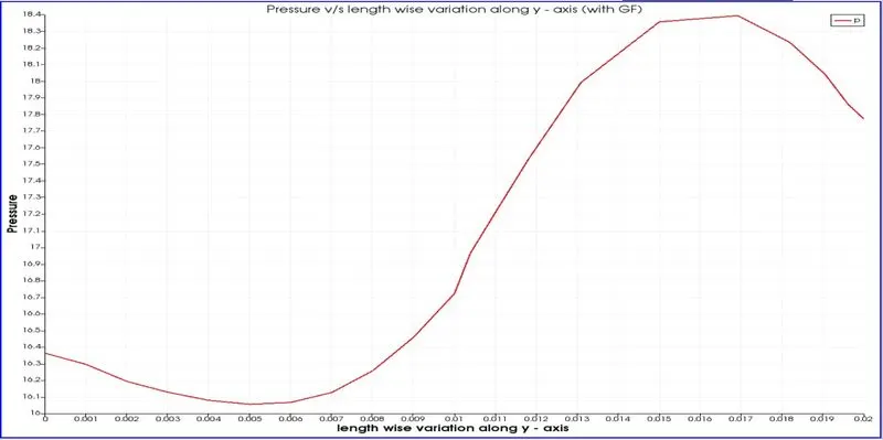
• By comparing the four graphs of velocity and pressure for two case, we can say that for the case 2 graphs there are many jerks in between, but the case 1 graphs are looking smooth in nature and this is due to the grading factor in case 2.

CASE-1: velocity layout for GF = 1

This layout can be done by using the "gylph" option

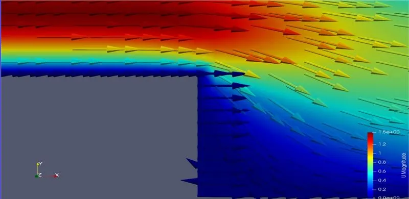
CASE-2: velocity plot for GF 0.2 and 5

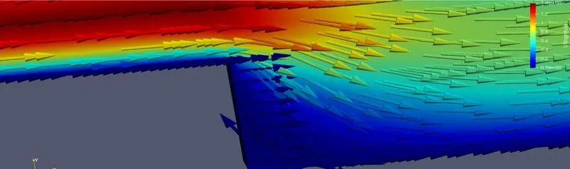
• From the two graphs we can say that back step is captured in the case 2 because grading factor is introduced and in case 1 we cannot see that properly because mesh is not refined and this happens due to the sudden expansion in the structure.
• Here we cannot see the thing exactly because when i paste the picture overhere some amount of clarity is lost.