Challenge

Week 8 - Simulation of a backward facing step in OpenFOAM

AAniket Bhaskarwar21 Dec 2021

Aim:

To simulate an incompressible-laminar-viscous flow through the backward facing step geometry in OpenFOAM.

Solution

I. Introduction

The separation and reattachment of flows is an important process in a large number of practical engineering configurations like separation of flow behind vehicles, flow behind flame holders in combustors, separated flow in diffusers, and separation bubbles on airfoils, inlet tunnel flow of engine or inside a condenser/combustor. In such flows presence of recirculation zone affects the heat, mass, momentum, transport processes. In order to design such configurations it becomes very important to predict these complicated flows and is achieved by understanding the behavior of reattaching flows [2]. Among two-dimensional flow the backward-facing step is considered simplest reattaching flow. It is also called as ‘step flow’ as a step expansion in flow direction causes a flow to separate. The separation line is almost straight and fixed at edge of step so it creates only one separation region not two , i.e behind the step. And also the streamline upstream are almost parallel to wall at separation point so the influence of upstream occurs only downstream of separation [1]. This makes a simple geometry like backward facing step, more convenient to predict the separating and reattaching flows.

The fluid flow takes place from upstream of step where flow is fully developed and uniform with parabolic velocity profile. When fluid flows past the step due to its high momentum flow is unable to follow the geometry well and end up reattaching to the wall after some distance in downstream of step. The ﬂow ﬁeld of Backward Facing Step is generally divided into four regions [2]: a separated shear layer, the recirculation region under the shear layer, the reattachment region, and the attached or recovery region as shown in figure 1.

Separated shear layer

The upstream viscous boundary layer separates at sharp corner forming a free-shear layer. The point where the gradient of velocity component which is parallel to the wall becomes zero, the boundary layer separation occurs. This flow separation happen only if there exist viscosity induced boundary layer and adverse pressure gradient in flow direction which is enough strong to overcome momentum of incoming fluid. If formed boundary layer is laminar , transition may begin soon after separation [1]. This separated shear layer in first half part just downstream of separation is much of same like ordinary plane mixing-layer.

Mixing Layer: A separating stream line which is the separating line between mainflow which is decelerates due to sudden expansion and a recirculation region. The separating stream line is the location of very high velocity gradient called ‘mixing layer’. This high velocity gradients inflects the mean transverse velocity profile which leads to Kelvin-helmholts instabilities ( due to velocity shear ) which forms a coherent turbulent structures that get shed from the layer and advected along shear layer.

As this separated shear layer moves further downstream, it approaches bottom wall with increasing angle in reattachment zone and impinge on the wall. This re-attaching shear layer differ from plane mixing layer in the respect that the flow on low speed side of shear layer highly turbulent [5]. Due to strong adverse pressure gradient the part of impinged shear layer fluid is deflected upstream into recirculating flow. This shear layer in the reattachment zone is now subjected to adverse pressure gradient and strong interaction with wall. Due to one or more of these mechanism the rapid decrease in Reynolds normal and shear stresses takes place. The velocity profile stabilizes at certain length in downstream.

Recirculation Region:

As flow reattaches with the wall at some distance downstream of step, the region of re-circulating flow is formed just below the separating shear layer. This recirculation zone cannot be characterized as dead zone, the literature tells that the maximum backflow velocity is usually more than 20% of free-stream velocity with significant value of negative skin friction coefficient [5]. This zone is region of null discharge with positive stream-wise velocity near separating stream line. And negative reverse velocity near side wall. This region can be considered as loss of energy as it is not taking part in main flow.

Reattachment Region:

Reattachment location is the point where separated shear layer reattaches to the surface. The literature gives two widely accepted definitions of reattachment point. The one defines it as the point where surface velocity (time averaged stream-wise velocity component measured very close to surface) equals to zero. The second defines it as a point where surface flow moves upstream 50% of the time [6]. Both definition yields same result with no appreciable difference. This reattachment length also be used as measure of entrainment from the separated shear layer. Few research article tells that in backward facing step flow the large scale vorticle structures develop between main flow and recirculation region owing to instabilities emerging in the separated shear layer, passes through reattachment point which results in oscillation of point of reattachment. This low frequency oscillations of reattachment length of primary recirculation region caused by impingement of eddies on reattachment is called flapping of primary reattachment line [5]. This may affect the region where flow stabilizes and original velocity profile is regained downstream.

Figure 1, shows the schematics of flow development on backward facing step.

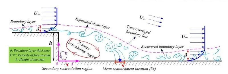
Figure 1: SChematic of BackwardFacing Step flow evolution [2].

The flow field downstream of flow is affected by Reynolds number of flow, the incoming initial velocity profile, step height, expansion ratio, adverse pressure gradient, length available downstream. Based on experimental investigation of flows in literature, gives Reynolds number range for different flow regimes, as Laminar (ReD < 1200), transition (1200 < ReD < 6600), turbulent (ReD > 6600) [1]. It was also observed that the two-dimensionality of flow was disturbed for Re > 400 , which lead to variation of velocity in spanwise direction (3^rd dimension) and flow becomes three-dimensional. Two dimensional simulations starts to underpredict primary reattachment length for Reynolds number beyond which actual flow is observed to be three-dimensional [4].

In the present analysis the flow is simulated in laminar regime with ReD = 1000, considering fully developed (delu/delx =0 ) parabolic velocity profile upstream of step. The inlet velocity is obtained from the hydraulic diameter based Reynolds number (ReD) considering incompressible fluid.

Density = 998 kg/m^3 , dynamic viscosity = 1.002e-3 kg/m-s , kinematic viscosity = 1.004e-6 m^2/s , Dh = hydraulic diameter = 4Ac /P = 4*h*1/2(h+1) = 4*1*1/2*(1+1) = 1

Re = 1000 = `(rho*U*Dh )/ (mu)` , The velocity obtained is 0.001 m/s.

II. Flow channel Geomtry

The geometry of the ﬂow conﬁguration is as shown in ﬁgure 2. it consists of a plane channel with a sudden stepwise expansion of the cross-section. The height of the channel in front of the step is h. Downstream of the step the channel height is given by H = h + S, where S deﬁnes the step height. An expansion ratio r = H/h=1+S/h =2. The computational domain has an extension of Lu and Ld in Upstream and downstream of the step, respectively. Lu is chosen in such a way that upstream length should not influence on the predicted results past the step, it was found that Lu >= 5h , five times the step height. In this case Lu is taken 8h which insures no influence of upstream on downstream. The downstream length (Ld) of computational domain is about 12h to get flow to be fully developed again, so simple outflow conditions are assumed as zero gradients (Neumann condition) of all flow variables.

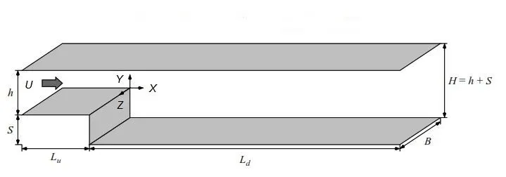
Figure 2: The ﬂow conﬁguration and the deﬁnition of length scales [1].

The study is focused on understanding the flow field in two-dimension only i.e the span-wise effects are not to be considered in the simulations. So the width of channel ‘B’ here is taken as h. The influence of side walls is not considered, as main objective of study is to get sense of flow development through the velocity profiles in some critical regions and effect of change in grid size.

III. Grid

A suitable computational grid is need to be chosen which suﬃciently resolves the critical regions of the domain, such as the boundary layers , the evolving free shear layers, recirculation region. In order to see the desired phenomenon in particular region of interest the grid size need to be kept small so to achieve this, in OpenFOAM the concept of ‘grading’ is used. So,

Grading factor (f) is ration of length of end cell to the start cell.

f = Length of end cell / length of start cell.

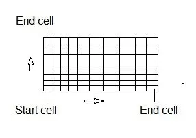
Figure 3: Start and end cell

The direction in which cells are considered will decide which cell to consider start or end cell as shown in figure 3 and the direction chosen will remain same for all cells. The cell can be graded in either of direction or in both directions. The f < 1 gives size of end cell less than start cell and f > 1 gives size of end cell greater than start cell.

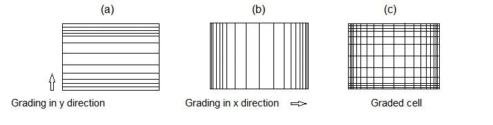
Figure 4: Grading in x and y direction.

The region very near to wall both in upstream and downstream, where the boundary layer developes is resolved using grading in y direction. The physics starts developing in the region of sudden expansion, so the region near the step is resolved using grading in x direction so that very small grid sizes can be maintained. The recirculation zone is another site which needs good amount of resolution in both directions i.e combined effect of grading in x and y direction. The grading in x direction , y direction and combined effect of both looks like as shown in figure 4 (a), (b) and (c).

In figure 4(a) while grading in y direction, for bottom side of cell value of f can be any value greater than 1 and for top side f need to be taken any value less than 1. Similarly for grading in x direction, for left boundary of cell the value of f can be any value greater than 1 and for right boundary of cell the value of f can be any value less than 1

The figure 5(a) & (b) shows the computational grid used for the simulation of backward facing step with and without grading respectively.

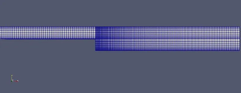
Figure 5(a): Computational grid with grading for simulation of backward facing step.

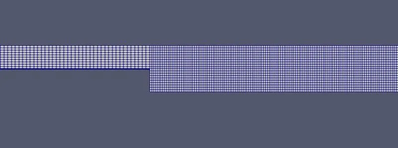
Figure 5(b): Computational grid without grading for simulation of backward facing step.

IV. Simulation Cases

In order to visualize the effect of grading on the quality of results two simulations cases are run. First simulation is based on the grid which is sufficiently fine in desired regions to capture the velocity profile properly and second simulation uses grid of same size everywhere with equal number of grid points as that of first simulation. Both simulation have 200 nodes in streamwise direction and 20 cells in y direction

V. Steps

The backward facing step flow is simulated using openFoam a open source software. The following steps are needed to perform simulation.

Choosing Solver
Creating geometry
Meshing
Problem setup – initial BC , Boundary condition
Post-processing – plotting results

1 . Choosing solver:

In openFoam the suitable case is choosen and made desired changes in it. The fluid used is a Newtonian fluid and is incompressible in nature with initial flow profile to be maintain as laminar. The icoFoam solver is chosen which is a incompressible solver in which cavity problem is taken as base case in which files are modified for geometry, boundary and initial conditions.

Creating geometry and Meshing:

The flow domain for the for simulation is as shown in figure 6. This domain need to be created in the openFoam environment.

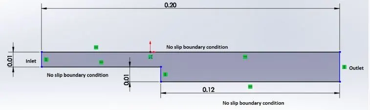
Figure 6; Flow domain

The BlockMeshDict file is used to create geometry over which flow is simulated and meshing of that geometry. The BlockmeshDict file used for the simulation is given:

_____________________________________________________________________

/*--------------------------------*- C++ -*----------------------------------*
========= |
/ F ield | OpenFOAM: The Open Source CFD Toolbox
/ O peration | Website: https://openfoam.org
/ A nd | Version: 8
/ M anipulation |
*---------------------------------------------------------------------------*/
FoamFile
{
version 2.0;
format ascii;
class dictionary;
object blockMeshDict;
}
// * * * * * * * * * * * * * * * * * * * * * * * * * * * * * * * * * * * * * //

convertToMeters 0.01;

vertices
(
(0 0 0) // vertex0
(8 0 0) // vertex1
(8 0.5 0)// vertex2
(0 0.5 0)// vertex3
(8 1 0)// vertex4
(0 1 0)// vertex5
(20 1 0)//vertex6
(20 0.5 0)//vertex7
(20 0 0)//vertex8
(20 -1 0)//vertex9
(8 -1 0)//vertex10
(0 0 1)//vertex11
(8 0 1)// vertex12
(8 0.5 1)// vertex13
(0 0.5 1)// vertex14
(8 1 1)// vertex15
(0 1 1)// vertex16
(20 1 1)//vertex17
(20 0.5 1)//vertex18
(20 0 1)//vertex19
(20 -1 1)//vertex20
(8 -1 1)//vertex21

);

blocks
(
hex (0 1 2 3 11 12 13 14 ) (50 5 1) simpleGrading (1 5 1)
hex (3 2 4 5 14 13 15 16 ) (50 5 1) simpleGrading (1 0.2 1)
hex (2 7 6 4 13 18 17 15 ) (150 5 1) simpleGrading (5 0.2 1)
hex (1 8 7 2 12 19 18 13 ) (150 5 1) simpleGrading (5 5 1)
hex (10 9 8 1 21 20 19 12 ) (150 10 1) simpleGrading (5 10 1)

);

edges
(
);

boundary
(
inlet
{
type patch;
faces
(
(0 11 14 3)
(3 14 16 5)
);
}
outlet
{
type patch;
faces
(
(6 17 18 7)
(7 18 19 8)
(9 8 19 20)
);
}

walls
{
type wall;
faces
(
(4 5 16 15)
(0 1 12 11)
(6 4 15 17)
(10 9 20 21)
(10 21 12 1)

);
}
);

mergePatchPairs
(
);

// ************************************************************************* //

______________________________________________________________________________

In first part the vertices are defined which makes the geometry as shown in figure 7. The first vertex , vertex 0 is considered as origin. Vertex 1 the second vertex is defined in such way that, vector going from 0 to 1 shows the local x- axis. Similarly the vertex 2, the third vertex shows the vector going from 1 to 2, which is the direction of local y-axis. After defining vertex 3 i.e the fourth vertex, 0,1,2,3 together will define one plane. This local directions are important which helps openFoam to understand what are x,y,z direction and how the surfaces are oriented so that with connection of each vertex it will form the desired geometry.

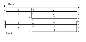
Figure 7: Defining verties

After the vertex are connected to form a geometry the next part will help to mesh it. OpenFoam divides whole geometry into various blocks. Each block is meshed individually with different number of cells and with different grading factor as the natire of problem demands.

hex (0 1 2 3 11 12 13 14 ) (50 5 1) simpleGrading (1 5 1)

hex denotes the hexagonal elements, the numbers in bracket tells openFoam rom which vertex that block is created, followed by second bracket (50 5 1) which tells the openFoam the number of cells we nned in the x , y and z – directions. SimpleGrading will control the stretching of mesh in the respective directions.

In third part the boundaries are defined to let openFoam know which are inlet, outlet and walls of the geometry.

boundary
(
inlet
{
type patch;
faces
(
(0 11 14 3)
(3 14 16 5)
);
}

So,

Patch – surface that exchanges the mass.

Wall – surfaces wich do not transfer any mass.

Empty – Where no calculation are done .

That is why, Inlet and outlet are defined with type ‘patch’ and value as ‘faces’ with respective vertices defining that particular face. This faces are defined in such a way that the normal to one surface do not intersect with normal of other face i.ethe normal always point outward, generally they are defined as per right hand rule. The fingers of right hand are curled and thumb is stretched outward which shows the direction of outward normal to surface as shown in figure 8.

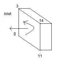
Figure 8: Defining face types using right hand rule.

The faces which are not defined the openFoam will consider them as ’empty’. After making desired changes in BlockMeshDIct file the file is run first by – executing ‘blockMesh ’ [at ‘ 0 constant system ‘ level].

3. Problem Setup:

This defines the initial and boundary conditions for Velocity and Pressure, the files are locates in ‘0 folder’.

_____________________________________________________________________

Internalfields uniform (0 0 0) – indicates the initial condition. Value of velocity at inlet here is taken as (1 0 0) which shows 1 m/s is defined only in x direction

At outlet – it is defined as ZeroGradient which indicates the values are velocity are extrapolated from the values of internal nodes points i.e Neumann Boundary Condition. At walls the no slip conditions is assumed.

For pressure , The outlet pressure is kept atmospheric i.e uniform 0 indicates the gauge pressure of zero and inlet pressure values are extrapolated from the adjecent node values obtained from solution of pressure field.

________________________________________________________________

_____________________________________________________________________

The constants used for simulations are defined in constants file.

_____________________________________________________________________

__________________________________________________________________________

The another important file that control the simulation is ControlDict file. This file controls the simulation time and also the time step value. The suitable inputs are given to the file to control the simulation.

Simulation time is calculated as :

Time = distance / Speed i.e Domain length/ speed of fluid

Time = 0.2/0.001 = 200 seconds

And dt is chosen as 0.01.

_______________________________________________________________

_______________________________________________________________________

After making changes in these files the simulation is ready to run . The simulation is run by executing, ‘icoFoam’ followed by key. After completion the results are post process in ‘paraview’ and is opened by executing ‘paraFoam ’.

4. Post-processed Results:

Simulation 1:

The simulation is carried out using mesh with grading in x and y direction. The mesh looks like as shown in figure 9:

Figure 9: Computational grids used for the simulation of the backward-facing step ﬂow.

The velocity distribution obtained from simulation is as shown in figure 10:

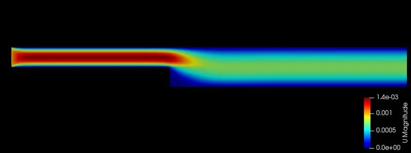
Figure 10: The velocity distribution

This shows the velocity upstream step is higher as compared to velocity downstream of step which is consequence of adverse pressure gradient developed in streamwise direction due to sudden change is area i.e expansion.

The step flow are characterized by a existence of recirculation zone at corner just downstream of step as shown in figure 11:

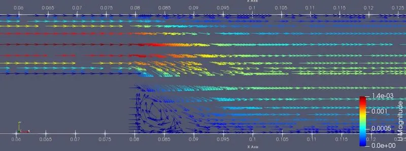
Figure 11: The Recirculation region

The velocity magnitude in this low pressure region is very small as compared to region just adjacent to recirculation bubble as this region consist the separated shear layer moving relatively faster. In this region the velocities are negative where the flow is turning in upstream direction followed by positive velocities as flow take turn again in streamwise direction. In the case of the primary recirculation region, it is mainly the rotational movement of the shear-layer vortices impinging on the lower channel wall which is causing the zones of negative ﬂuid velocity. Figure 11, also helps in prediction of reattachment point which approximately lie in between X= 0.085 m and X= 0.090 m. The close view of this zone is shown in figure 12.

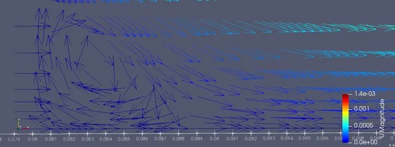
Figure 12: Close view of recirculation region.

Figure 13: depicts the velocity profile at different positions (X) . Over a long distance downstream the step, the main flow moves between the upper channel wall and the primary recirculation region. The flow is confined by the wall and the separation bubble in such a way that the velocity profile changes very little from step (0.08m) to X =0.085m by 14% in maximum velocity magnitude. As flow moves further downstream the area of main flow increases as consequence, due to mass conservation the maximum velocity decreases.

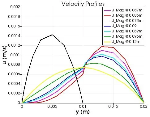
Figure 13: Proﬁles of the ﬂow velocity at diﬀerent streamwise positions

Now the momentum of flow is now confronted by adverse pressure gradient more aggressively. A streamwise pressure gradient is present which decelerates the flow to reduce the maximum velocity so that the velocity profile becomes a parabolic again. The figure 14 shows the the downstream of recirculation region , the pressure level are significantly higher than upstream.

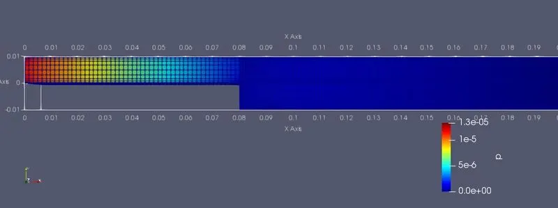
Figure 14: Pressure gradient along the backward facing step.

The velocity profiles also helps to predict the location of re-attachment point where separated shear layer re-attaches the wall. The location where the streamwise component of velocity changes the sign very near to wall [6], the reattachment point lies in between that locations. The figure 15(a) and (b) shows variation of streamwise component of velocity at two different locations.

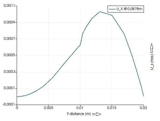
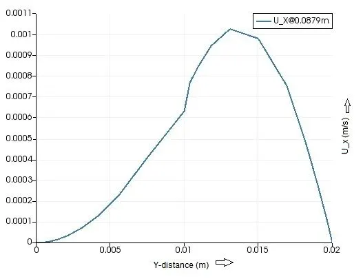
Figure 15(a): Stream-wise component of velocity at 0.0878 m.

At location 0.0878m downstream of step and 0.009 m from bottom of step the velocity is negative and 0.0879 m downstream of step and 0.009m from bottom os step the velocity is positive as shown in table 1. So the flow reattaches between 0.0878 m to 0.0879 m downstream.

Table 1: U_x magitudes

	0.0878 m	0.0879 m
U_x @ - 0.0099m	-1.05e-8	1.31e-8

Simulation 2:

The simulation is carried out using mesh with no grading in x and y direction. The cell stretching is same everywhere. The mesh looks like as shown in figure 16.

Figure 16: Computational grids used for the simulation of the backward-facing step ﬂow.

The velocity distribution obtained from simulation is as shown in figure 17 :

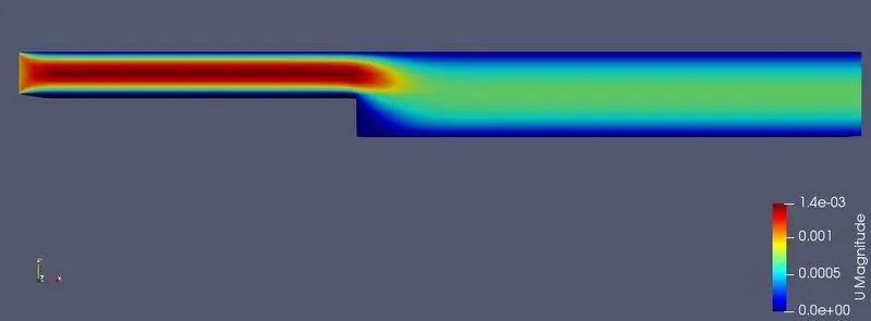
Figure 17: The velocity distribution

Velocity distribution is same as discussed earlier but the differences in the values at same respective points will start to become significant as these region of importance are not refined sufficiently. This difference can be seen at peak value of velocity in upstream as compared to the value of centerline velocity of upstream in case of graded mesh. The figure 18, shows the velocity distribution just upstream of step.

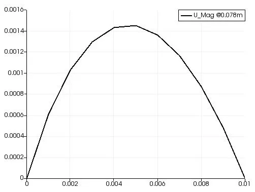
Figure 18: velocity profile at 0.078 m

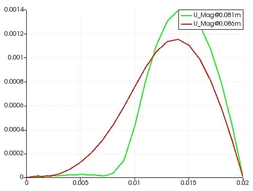
Figure 19: Velocity profiles in downstream of step

The velocity distribution at downstream of step is shown in figure 19. At 0.081m for lower region (Y=0 to Y = 0.01) the velocity shows ups and downs due to recirculation in that region.

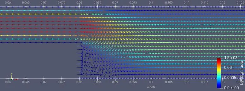
Figure 20: Recirculation region

The recirculation zone is shown in figure 20. The insufficient resolution also results in little deviation of reattachment location which is in between X = 0.0874m to X=0.0875 m, from graded mesh configuration.

Simulation 3:

The grid is made finer by increasing the number of cells in stream-wise direction to 576 [1]. The dt was taken here as 0.001 with total simulation time of 20 sec. The maximum courant number of 0.0268. The maximum velocity just upstream of step is 0.001425 m/s which is somewhat near to the value predicted by the simulation 1 with graded mesh having 200 cells in stream-wise direction. The reattachment point is found to be in between X = 0.0858 m to X = 0.0859m where the separated shear layer reattaches to the wall.

VI. Conclusion

In this simulation the flow in the downstream of step looks very simple with only one circulation region at corner very near step, but in real the downstream flow structure is extremely complex with multiple recirculation zones which are continuously interacting with vertical structures emerging from the separated shear layer which can be seen in the present simulation as flow field is solved using laminar solver which do not take turbulence in account. Turbulent models like LES and RANS will give more accurate results close to reality.
The grading results in refining particular region as per developing physics and the graded mesh shows deviation in values from the mesh with no grading (GF =1 everywhere).
The fine grids with more numner of cells in respective directions will impart more accuracy in prediction flow field behavior and Primary, Secondary recirculation regions. the simulaion 3 is carried out with 576 number of cells in x direction results in similar behavior of flow but with difference in values which are more accurate.

Reference

Schafer, M. Breuer and F. Durst, The dynamics of the transitional ﬂow over a backward- facing step, J. Fluid Mech. (2009), vol. 623, pp. 85–119.
Lin Chen, Keisuke Asai, Taku Nonomura , Guannan Xi Tianshu Liu, A review of Backward-Facing Step (BFS) ﬂow mechanisms, heat transfer and control, Thermal Science and Engineering Progress 6 (2018) 194–216.
S. Onur and E. Baydar, Laminar channel flow over a square step, International Journal of Engineering Science Vol. 30, No. 9, PP. 1109-1116, 1992
Biswas, M. Breuer F. Durst, Backward-Facing Step Flows for Various Expansion Ratios at Low and Moderate Reynolds Numbers,ASME, Vol. 126, May 2004.
K. Eaton and J. P. Johnston, A Review of Research on Subsonic Turbulent Flow Reattachment, AIAA Journal, VOL. 19, NO. 9, September 1981.
Chiang Shih, Chili-Ming Ho, Three-Dimensional Recirculation Flow in a Backward Facing Step, ASME, 116, June 1994

Week 8 - Simulation of a backward facing step in OpenFOAM

Ship work like this
in your own course.

Talk to a career counsellor

Ship work like thisin your own course.

Talk to a career counsellor

Ship work like this
in your own course.