Week 4 - CHT Analysis on Exhaust port

Aim

Perform CHT Analysis on Exhaust Port.

1. Give a brief description of why and where a CHT analysis is used.
2. Maintain the y+ value according to the turbulence model and justify the results.
3. Calculate the wall/surface heat transfer coefficient on the internal solid surface & show the velocity & temperature contours in appropriate areas.
4. How would you verify if the HTC predictions from the simulations are right? On what factors does the accuracy of the prediction depend on?

Solution

CHT simulation can solve flow and heat transfer in both fluid and solid regions simultaneously. It can be used where the heat is transferred at fluid solid interface. CHT analysis can predict more accurate results as equation’s for solid and fluid are solved simultaneously. CHT also have advantage that it can display solid region information.

1. Computational Domain and Mesh

The computational domain comprises of 4 inlet sections through which the heated gas from the engine enters into Exhaust Port assembly which connects to the curved exit section which connects to the inlet of Catalytic Converter as shown in figure 1 . The entire computational domain is discretized with triangular mesh elements.

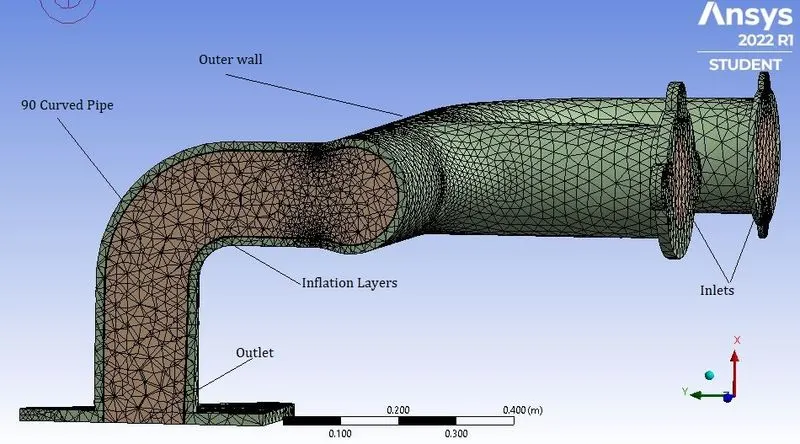
Figure 1 Mesh

The mesh details are shown in figure 2. The element size of 50mm was used with the 10 inflation layers of growth Rate 1.2.

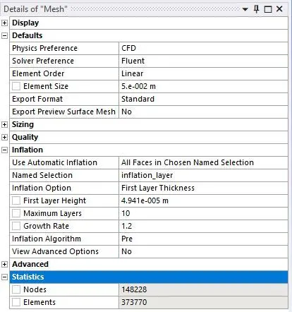
Figure 2 Mesh Details.

In order to understand heat transfer from fluid to the solid it is important to resolve viscous sub-layer ( y⁺ < 5 ). The first layer of thickness ( y ) is the distance of first cell from the wall and it should be such that first cell happen to be In viscous sub layer to take viscous effects into account for correctly predicting the surface heat transfer coefficient.

• The first layer of thickness is calculated considering y⁺ = 0.8 (Recommended value for viscous sub-layer is y⁺≤ 1 [Ansys documentation] ).

For analysing the flow behaviour in curved outlet limb, the temperature and velocity measurements at different cross-sectional planes were numbered from 0 to 5. For the curved pipe, the four sections of the 90 curved part were numbered by S1-0, S1-30, S1-60, and S1-90. The remaining cross-sections were numbered by S0 at upstream of bend and S-2, S-3, S-4, and S-5 at downstream of bend as shown in figure 3.

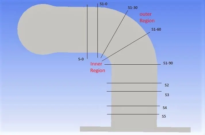
Figure 3 Geometry

2. Boundary Conditions

• The hot air of 400^o C with 20m/s enters into exhaust port assembly and the outlet boundary condition was set at an ambient pressure 101.325 kPa.
• The interface wall boundary condition was used on inner wall of pipe, which is surface between solid and fluid domain. For fluid domain side of the interface wall the velocity and temperature law of the wall were applied. For the solid domain side of interface wall the No-slip boundary condition was applied on the wall.
• The constant wall temperature thermal boundary condition, the constant wall heat flux thermal boundary condition are widely used outer wall boundary conditions. But in this simulation the third type of wall boundary condition is used for which the heat transfer coefficient and far-field temperature are defined. The automotive exhaust system are directly exposed to the environment. Therefore, this wall boundary condition can reveal the flow and heat transfer behaviour of exhaust pipe.
• The far-field temperature was 298.15 K, and the heat transfer coefficient of this boundary was set to be 20 W/m² K. The outer wall temperature of the system was set at 300 K.

3. Physical Aspect

The turbulence in the flow was predicted using k-omega SST model. K-epsilon model have strong tendency to miss or under-predict separation under adverse pressure gradients and also it do not performs well in predicting near wall behavior. Furthermore k-omega model performs well in near wall region under mild pressure gradients but is very much sensitive to free stream turbulence condition which may result in over-predicting the wall shear stress i.e skin friction coefficient.

• Therefore, the k-Omega SST deals with these limitations by merging the merits of k-Omega and k-epsilon. The blending function allows k-omega SST to behave as k-epsilon in far stream where it performs well and in near wall region it behaves as k-omega which efficiently communicates the wall presence to the flow without a need for additional transport equations or damping functions.
• In this problem it is very necessary to resolve the near wall region to predict the heat transfer coefficient values. Fluid also flows through various curved pipe sections where the adverse pressure gradient is induced due to curvature which tends to separate the core which affects the heat transfer characteristics of the region at bend. Due to mixing of four fluid streams at outlet pipe entrance makes the flow sensitive to free stream turbulence. These key characteristics makes k-omega SST as a reasonable choice for simulating the turbulence. The need to resolve viscous sub-layer limits the value of y⁺ less than or equal to 1.

Pressure based solver is used as working fluid is incompressible in nature with steady state approach.

Dean Number:

For the fluid flow characteristic of a curved pipe, Dean first theoretically analyzed laminar flow in a curved circular-sectioned pipe. It was found that the two symmetrical counterrotating vortices were produced as a secondary flow structure as effect of curvature. These vortical structures were named as Dean vortices. The Dean number used to characterize curved flows was first proposed by Dean.

• Dean number is ratio of centrifugal force to the viscous force which depends on curvature ratio and flow Reynold’s number.

`De = Re sqrt(D/(2Rc))`

In present study, air was taken as working fluid which entered at 673 K and 20 m/s. The inlet diameter was 0.166 m with outlet diameter of 0.150 m.

• Properties of Air@ 673K was taken from standard Heat and Mass Transfer Data Book: `rho`= 0.524 kg/m³ µ= 33.05 e‑6 kg/m s Cp= 01067 j/kg K k= 0.05210 w/m K `Tunderset(solid)`= 298 K `Tunderset(ambient)`= 298K
• R at bend(radius of curvature): Rin = 0.05 m, Rout = 0.25, Rc = 0.15 m.
• De= 3.9155e+4, Re = 52638, Pr= 0.678, y (Thickness of first cell)= 4.94e-55 m (0.0494 mm)

Results:

Fluid at 20^o C and 673 K enters through four parallel inlets where it mixes together at the entrance of exit limb to form a one stream of fluid. Where fluid accelerates while passing through the bend section in order to keep mass flow rate conserved. This acceleration of fluid in bend significantly affected the heat transfer behaviour of system. The flow at the entrance of curved pipe becomes fully turbulent due to mixing of streams together, the velocity distribution along xz-plane as shown in figure 4. The uniformity in a velocity is attained due to mixing at entrance of curved pipe.

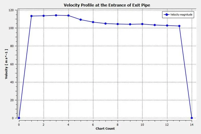
Figure 4

Velocity and temperature distribution at the upstream section of the curved part affected due to presence of curvature that shifted the streamwise velocity core to the inner side as shown in figure 5. At the curvature, due to centrifugal force the fluid core got detached from the inner side. Therefore, this high temperature core in air flow impinged on the outer side, little downstream of bend due to its high momentum.

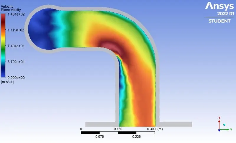
Figure 5

After S1-90, due to curvature induced pressure gradient in just downstream of bend and over the top of it the centrifugal effect made this boundary layer to separate from the inner wall. This separation resulted in the low pressure recirculation zone beyond the point of separation. This fluctuating and growing low pressure wake region is as shown in figure 6. The recirculation here is very small so effect of it on downstream flow is somewhat neglected.

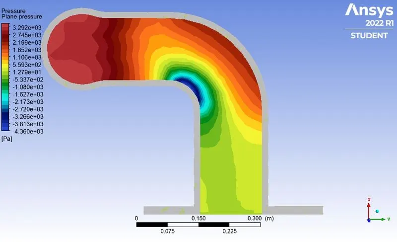
Figure 6

The direct contact of high-temperature core to outer region resulted in increased wall temperature. Therefore, the heat transfer to the outside of the pipe was further enhanced by the temperature difference between the wall and the ambient. The stream-wise temperature distribution along the central XY plane is as shown in figure 7.

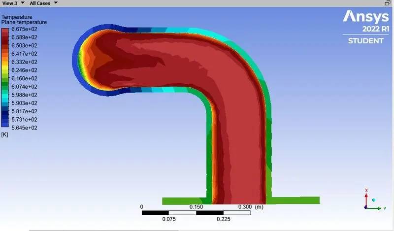
Figure 7

The separation of air after S1-90 resulted in a significant decrease in temperature of the air near inner wall, these low-temperature region near to the inner wall were shown in figure7, and the temperature difference between the inner wall and ambient decreased. Hence, the heat transfer was reduced at the inner wall after the curvature. It can be concluded that flow impingement enhanced heat transfer and flow separation suppressed the heat transfer.

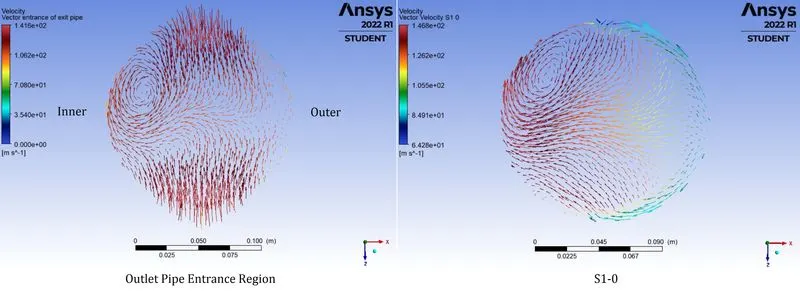
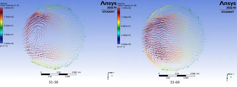
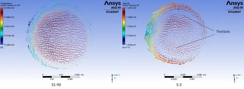
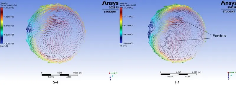
Figure 8

In this present study the Dean number happened to be 3.91e+4 with curvature ratio of 2. The strong centrifugal force exhibited the Dean vortices as shown in figure 8.

• At S1-90, the core of velocity slightly started shifting towards outer wall as impingement happen downstream of S1-90 so secondary flow have just started to take shape. At S-2 high velocity core started to diffuse towards outer wall pushing the parts of core in top and bottom part of section. As secondary flow developed in S-2, S-3 and S-4, the velocity core further shifted towards top and bottom as shown infigure 8. This movement promoted the mixing of air and enhanced heat transfer performance.

The Impingement and secondary flow development in downstream of bend shifted the temperature core towards the outer wall which is shown in figure 9. Colour contour for temperature core were obtained from CFD-Post-Processing.

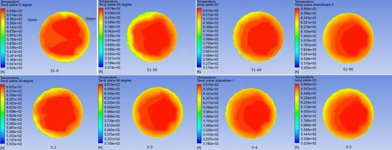
Figure 9

Radial Profiles of Velocity and Temperature for Various Cross-Sections

The profiles of velocity and temperature along different radial directions for the various cross-sections are depicted in figures 11 and 12, respectively. The three radial directions are defined as θ = 0^o, 90^o, 180^o from the pipe centre to inner, top, and outer wall as shown in figure 10.

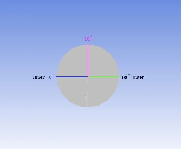
Figure 10

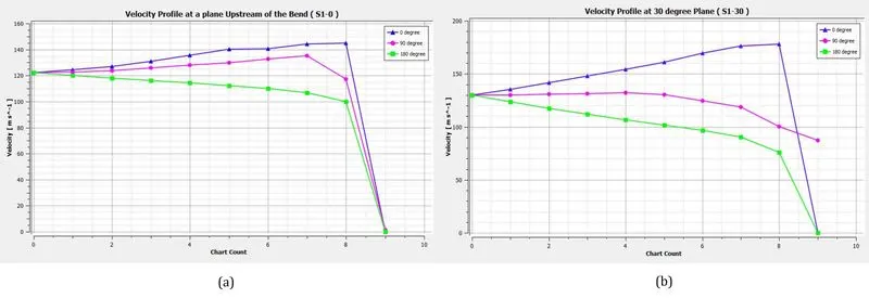
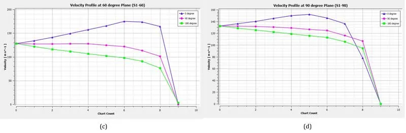
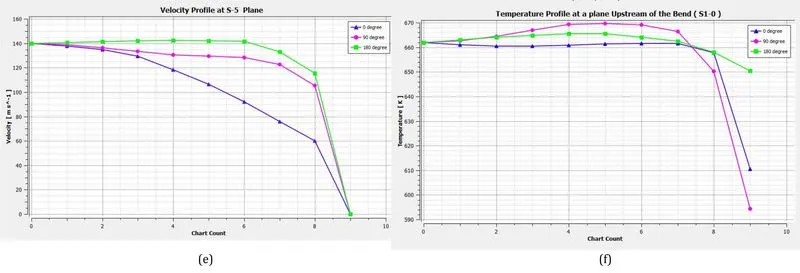
Figure 11

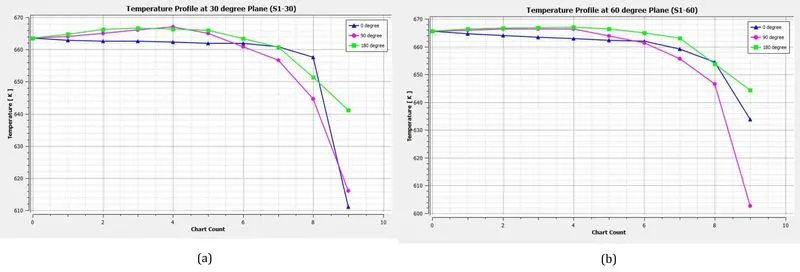
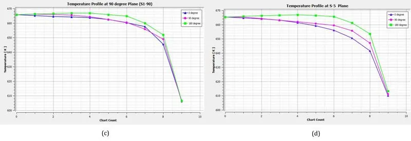
Figure 12

• At S1-0, due to mixing of fluid streams at the entrance there exists some non-uniformity in the flow at inner wall which reduces towards outer wall. This makes the velocity to fluctuate slightly as we move towards inner wall as shown in figure 11 which was consistent with figure 8. The higher velocities at inner wall region shows that velocity core is attached at inner wall. The Figure 11(f) shows that the temperature core was still evolving, at 0 (inner region), presence of mixing (in entrance region) induced vortical structure which was trying to create uniformity resulted in reduced temperature. For 90 (top) and 180 (outer) temperature increased as we moved away from centre towards surface but very near to surface temperature fell due to formation of low temperature regions which were consistent with figure 9.

• At S1-30, The curvature effect kind of changed the pressure distribution (figure 6) which shifted the velocity core towards inner side depicted by 0 degree curve in figure 11(b), increasing the magnitude of velocity as we moved towards the wall from centre with very much reduced velocity at top (90 degree curve) and outer side (180 degree curve). The temperature core slowly started its transition away from inner side toward outer side which can be seen from the temperature profile at 90and 180 degree in figure 12(a), this behaviour found to be consistent with figure 8.

• At S1-60, the velocity core was still attached but the velocity peak in velocity profile for 0 degree (figure 11) shifted little away from the wall which tells core was detaching. This effect made transitioning of temperature core more towards outer wall (figure 9), depicted by increasing trend in temperature at 180 degree line as shown in figure 12(b).

• At S1-90, velocity peak shifted away from inner wall with increase in velocity on outer and top wall as shown in figure 11(d). The flow has already separated creating a small wake close to inner wall which brought more mixing reducing the temperature near inner region as shown in figure 7.

• At S-5, the velocity and temperature core shifts on outer wall depicted in figure 11(e) and 12(d). After S1-90 the flow impinged on outer wall, increasing the temperature of outer side which increase the heat transfer to ambient. This heat transfer increased the temperature of the Outer-convection wall; in contact with ambient as shown in figure 13.

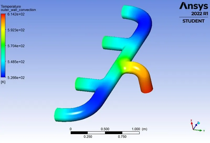
Figure 13

Nusselt Number

The Nusselt numbers talks about relatively the strength of Convection over Conduction heat transfer. This Nusselt number is function of Reynolds number and Prandtl number.

Nu = f (Re,Pr)

• From the results mention above it is clear that at and downstream of curvature flow accelerates i.e. the Reynolds number increases significantly in downstream. The distribution of velocity core on outer, top, and bottom side of pipe results in improved Re which proportionally enhances the Local Nu. High values of Nu suggested the further enhancement in Surface heat transfer coefficient at interface of fluid and inner pipe wall. Therefore, based on the flow deviation and impingement, along with the secondary flow formation, it was observed that the heat transfer performance improved. The area-average value of Surface Heat transfer Coefficient at the interface of fluid and the wall was 22.53 w/m² K.
• The Dittus-Boelter equation for fully developed turbulent flow is used for calculating Nu for straight pipe. But empirical relation for curved pipe can be obtain from Regression Analysis of experimental results.

The factors like Mesh quality, Selection of turbulence Model, y+ can affect accuracy of solution

Conclusion

• Owing, to the detachment from inner wall, impingement on outer wall as well as secondary flow development resulted in the temperature and velocity profiles in downstream of curved part (after S1-90) differed significantly from those of S1-0.
• Curvature effect accelerated the flow which got impinged on outer wall combined with formation of secondary flow structures that distributed temperature core to top and bottom side resulted in enhanced heat transfer.