Week 5.1 - Mid term project - Solving the steady and unsteady 2D heat conduction problem
Aim:
To solve the 2D steady & transient heat conduction equation by using the point iterative techniques.
1. Jacobi Method
2.Gauss seidel Method
3. Succesive over-relaxtaion Method
Solution:
The domain used for analysis is a unit square with a Dirichlet boundry condition on all faces.
The prescribed surface values of temperature are as follows:
Top Boundary = 600 K Bottom Boundary = 900 K
Left Boundary = 400 K Right Boundary = 800 K
The domain is now converted to a grid using m=n=10 number of points along x and y directions respectively as shown in figure.
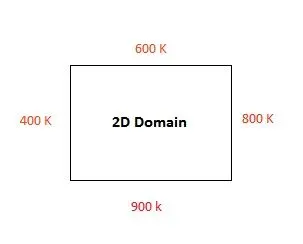
Fig. 1 Representation of 2D domain
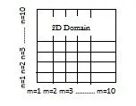
Fig.2 Representaion of 2D grid
Heat conduction equation is solved at each discrete point which ae spaced by Δx in x direction and Δy in y direction in this problem both are equal. Before solving
the steady and unsteady equation at each node these are to be discritized using implicit and explicit numerical schemes.
A. Steady state heat conduction equation:
The heat conduction eqauation in two dimension is written as:
`(delta T) / (delta tau)`= `alpha((delta^2T)/(delta^2x)+(delta^2T)/(delta^2y))`
When steady state the above equation boils down to :
`alpha((delta^2T)/(delta^2x)+(delta^2T)/(delta^2y))`= 0
1. Formulation:
The above equation is now discritized using finite difference method in which spacial terms are central in space.
The final discritized equation is:
`Toverset(n+1)i,j = `((T(i-1,j) + T (i+1,j) )k1 +(T(i,j-1) + T(i,j+1)) k2 ) / (2 (k1 + k2) )`
Here 'i' and 'j' represents the location of respective node.
2. Program:
MATLAB code is used to solve 2D steady heat conduction equation.
clear all
close all
clc

% Defining Mesh
m =10;
n =10;
L=1;
dx=L/(m-1);
dy=L/(n-1);


% Initialising
% Boundary Conditions

T=50*ones(m,n);  % Defining initial temp at all grid points
T(1,:)=900;
T(m,:)=600;
T(:,1)=400;
T(:,n)=800;
T(1,1)=650;
T(1,n)=500;
T(m,n)=700;
T(m,1)=850;

Told=T;         % Defining Told
k1=1/dx^2;      % Constants
k2=1/dy^2;

%%


iterative_solver=3

tol = 1e-4;    % tolerence

%% ____________________________________________________________________________

% Jacobi Method

if iterative_solver==1
    jac_iter=1 % Itereration counter variable
    error=9e9  % Errror definition

%Convergence Loop

    while(error>tol)

        % space Loop

        for i=2:m-1
            for j= 2:n-1
            T(i,j)= ((Told(i-1,j)+Told(i+1,j))*k1 +(Told(i,j-1)+Told(i,j+1))*k2)/(2*
            (k1+k2));
            end
        end


          error = max(max(abs(T-Told)))  % error = max(abs(T-Told))  max(2Darray) = 1D
                                           array. Hence we need to use one more max.
          Told=T                         % Updating values of Told for next iteration
          jac_iter=jac_iter+1;


    end

  % Plotting Results

 figure(1)
 contourf(T,'ShowText','ON')            % 'f' indicates 'fill'
 colorbar;
 colormap(jet);
 xlabel('X-cordinate');
 ylabel('Y-cordinate');
 title_x=sprintf('Number of Iteration=%d',jac_iter)    %'%d' will assign value
                                                         corrosponding to jac_iter
 title(title_x)

end


%% ____________________________________________________________________________

% Gauss-seidel Method

if iterative_solver==2
    error=9e9;
    gs_iter=1

% Convergence Loop

    while(error>tol)

        % space loop

        for i=2:m-1
            for j= 2:n-1
            T(i,j)= ((T(i-1,j)+Told(i+1,j))*k1 +(T(i,j-1)+Told(i,j+1))*k2)/(2*(k1+k2));
            end
        end


          error = max(max(abs(T-Told))) % error = max(abs(T-Told))  max(2Darray) = 1D
                                          array. Hence we need to use one more max.
          Told=T
          gs_iter=gs_iter+1;


  end

 figure(1)
 contourf(T,'ShowText','ON')
 colorbar;
 colormap(jet);
 xlabel('X-cordinate');
 ylabel('Y-cordinate');
 title_x=sprintf('Number of Iteration=%d',gs_iter)
 title(title_x)

end

%% _____________________________________________________________________________

% Succesive Over-Relaxation Method

if iterative_solver==3

 sor_iter=1;
 error=9e9;
 w=1.4;                      % Over-relaxation factor


    while(error>tol)
        for i=2:m-1
            for j= 2:n-1

                  T(i,j)= (1-w)*Told(i,j) + w*((T(i-1,j)+Told(i+1,j))*k1 +(T(i,j-1)+Told(i,j+1))*k2)/(2*(k1+k2));


            end
        end
            error = max(max(abs(T-Told)));
            Told=T;
            sor_iter=sor_iter+1;


  end

 figure(3)
 contourf(T,'ShowText','ON')
 colorbar;
 colormap(jet);
 xlabel('X-cordinate');
 ylabel('Y-cordinate');
 title_x=sprintf('Number of Iteration=%d',sor_iter)
 title(title_x)
end
The governing equation is solved using three iterative technique as jacobi method , Gauss-seidel method and succesive over-relaxtion method.
Single code gives output for three method just by changing value of 'iterative solver = 1/2/3' respectively and results are plotted.
3. Results:
i . Jacobi Method:
Plot shows temperature distribution using Jacobi iterative solver technique.
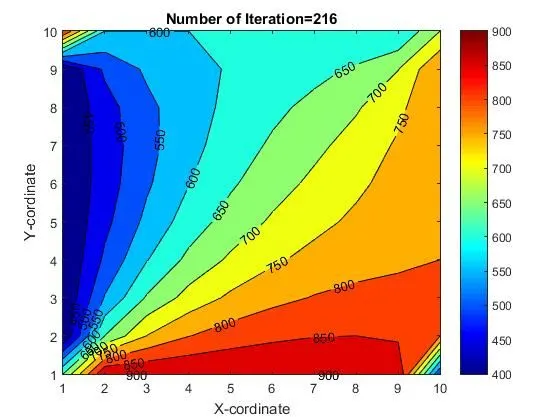
The number of iterations to get converged solution is 216.
ii . Gauss-seidel Method:
Plot shows temperature distribution using Gauss-seidel iterative solver technique.
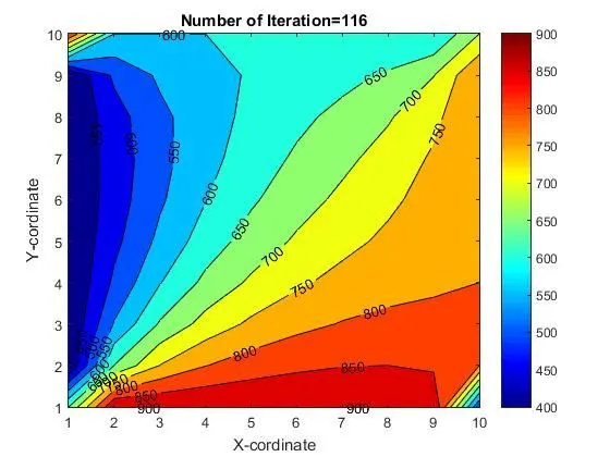
The number of iterations to get converged solution is 116. The use of new values from previous iteration resulting in significant
reductioin in number of iterations need to get converged solution.
iii . Succesive Over-relaxation Method:
Plot shows temperature distribution using Succesive over-relaxation iterative solver technique.
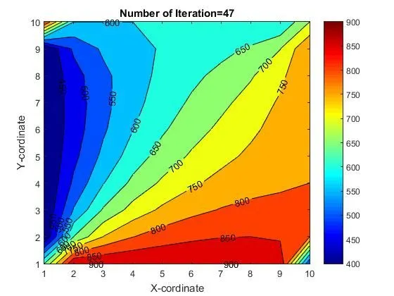
The number of iterations to get converged solution is 47. The solution is converging faster due to over relaxing factor of 1.4.
B. Unsteady state heat conduction Equation:
The unsteady/transient heat conduction eqauation in two dimension is written as:
`(delta T) / (delta tau)`= `alpha((delta^2T)/(delta^2x)+(delta^2T)/(delta^2y))`
Where `alpha` is Thermal diffusivity (`m^2/s`) is the property of material which shows ability to diffuse heat from the amount of heat that can be stored .
`alpha` = `k / (rho Cp)` = Thermal conductivity / Thermal storage per unit volume
Thermal diffusivity for metals is genarally small but in this calculations the diffusivity is assumed to be high to save computational time.
I. Explicit Scheme:
Formulation of explicit scheme is simple due to presence of terms whose values are known in eqauation. On other hand explicit scheme is very sensitive in terms of stability with little undesired deviation leads to a unstable solution. So stability of scheme is constrained by usage of very small time steps i.e more number of time steps to carry out calculation over a given time interal. But this limitation can be useful when the time accurate solution is desired as it provides high resolution.
1. Formulation:
The unsteady heat conduction equation in explicit form is :
`Toverset (n+1) i,j` =`Told(i,j) (1-2k1-2k2) + ((Told(i-1,j) + Told(i+1,j) )k1 +(Told(i,j-1) + Told(i,j+1)) k2 ) )`
Here 'i' and 'j' represents the location of respective node. k1 and k2 are contants.
k1= `1/(Deltax^2)`
k2= `1/(Deltay^2)`
2. Program:
MATLAB code is used to solve 2D unsteady heat conduction equation using explicit scheme.
clear all
close all
clc

% Defining Mesh
m =10;
n =10;
L=1;
dx=L/(m-1);
dy=L/(n-1);


% Initialising
% Boundary Conditions

T=20*ones(m,n); % Defining initial temp at all grid points
T(1,:)=900;
T(m,:)=600;
T(:,1)=400;
T(:,n)=800;
T(1,1)=650;
T(1,n)=500;
T(m,n)=700;
T(m,1)=850;
Told=T;
Tprev=T;


% Defining constants and variables
dt=0.1;
t=100;
nt=t/dt;
%alpha=20.34e-6 % alpha=k/pc (m^2/sec) thermal diffusivity, for pure iron block at 20 degree celcius, density=7897kgper m^3,specific heat=452 j/kgK, thermal conductivity k=72.7 w/mk

alpha=1e-2; %Reducing alpha increases computational time.
k1=(alpha*dt)/dx^2;
k2=(alpha*dt)/dy^2;
CFL=k1+k2;  %stability criterian CFL<0.5
tol=1e-4;

%% ____________________________________________________________________________________


iterative_solver=3


%% __________________________________________________________________________________

% Jacobi Method

if iterative_solver==1
  jac_iter=1;

  %Time Loop

   for k=1:nt
    error=9e9;

    %Convergence Loop

    while(error>tol)

        %Space loop

        for i=2:m-1
            for j= 2:n-1
                  T(i,j)= Told(i,j)*(1-2*k1-2*k2)+(Told(i-1,j)+Told(i+1,j))*k1 + (Told(i,j-1)+Told(i,j+1))*k2;
            end
        end
            error = max(max(abs(T-Told)));
            Told=T;  % Updating values of Told for next iteration
            jac_iter=jac_iter+1
    end
   end

% Plotting results
% Results shopuld be plotted outside convergence loop to capture converged results

 figure(1)
 contourf(T,'ShowText','ON')
 colorbar;
 colormap(jet);
 xlabel('X-cordinate');
 ylabel('Y-cordinate');
 title_x=sprintf('iteration=%d',jac_iter)
 title(title_x)
 pause(0.01)
end

%% ________________________________________________________________________________


% Gauss-seidel Method

if iterative_solver==2
  gs_iter=1;

  % Time loop

   for k=1:nt
    error=9e9;

    % Convergence Loop

    while(error>tol)

        %Space Loop

        for i=2:m-1
            for j= 2:n-1
                  T(i,j)= Told(i,j)*(1-2*k1-2*k2)+(T(i-1,j)+Told(i+1,j))*k1 + (T(i,j-1)+Told(i,j+1))*k2;  %T(i,j)= Told(or)T(i,j)(result wont change)*(1-2*k1-2*k2)+(T(i-1,j)+Told(i+1,j))*k1 + (T(i,j-1)+Told(i,j+1))*k2;
            end
        end
            error = max(max(abs(T-Told)));
            Told=T; % Updating values of Told for next iteration
            gs_iter=gs_iter+1;
    end
   end

 % Plotting
 % Results shopuld be plotted outside convergence loop to capture converged results

 figure(2)
 contourf(T,'ShowText','ON')
 colorbar;
 colormap(jet);
 xlabel('X-cordinate');
 ylabel('Y-cordinate');
 title_x=sprintf('Iteration=%d',gs_iter)
 title(title_x)
end


%% __________________________________________________________________________________


% Succesive Over-Relaxation Method

if iterative_solver==3
  sor_iter=1;

  %Time loop

   for k=1:nt
    error=9e9;
    w=1.5;

    % Convergence Loop

    while(error>tol)

        %Space Loop

        for i=2:m-1
            for j= 2:n-1
                  T(i,j)= (1-w)*Told(i,j) + w*(Told(i,j)*(1-2*k1-2*k2)+(T(i-1,j)+Told(i+1,j))*k1 + (T(i,j-1)+Told(i,j+1))*k2);
            end
        end
            error = max(max(abs(T-Told)));
            Told=T;
            sor_iter=sor_iter+1;

    end
    Tprev=T;
   end

%Plotting
%Results shopuld be plotted outside convergence loop to capture converged results

 figure(3)
 contourf(T,'ShowText','ON')
 colorbar;
 colormap(jet);
 xlabel('X-cordinate');
 ylabel('Y-cordinate');
 title_x=sprintf('Iteration=%d',sor_iter)
 title(title_x)
end
3. Results:
i . Jacobi Method:
The discritized eqaution using Jacobi Method is:
`Toverset (n+1) i,j` =`Told(i,j) (1-2k1-2k2) + ((Told(i-1,j) + Told(i+1,j) )k1 +(Told(i,j-1) + Told(i,j+1)) k2 ) )`
Here, old values are used everywhere for a given iteration.
Plot shows temperature distribution using Jacobi iterative solver technique.
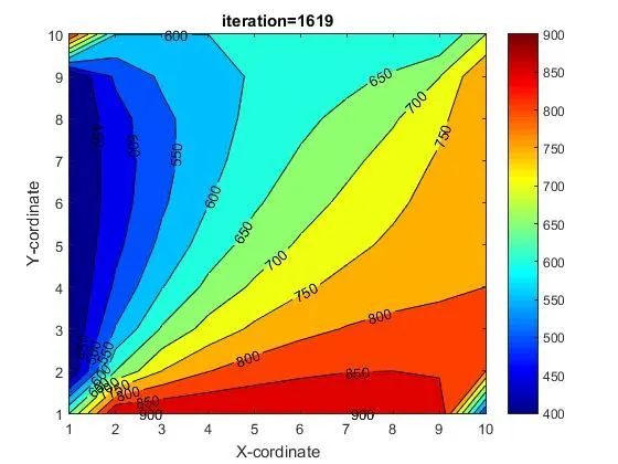
The number of iterations to get converged solution is 1619.
ii . Gauss seidel Method:
The discritized eqaution using Gauss-seidel Method is:
`Toverset (n+1) i,j` =`Told(i,j) (1-2k1-2k2) + ((T(i-1,j) + Told(i+1,j) )k1 +(T(i,j-1) + Told(i,j+1)) k2 ) )`
Here, updated values are used i.e Told is replaced by T as the new temperature values are being calculated in previous iteration.
Plot shows temperature distribution using Gauss-seidel iterative solver technique.
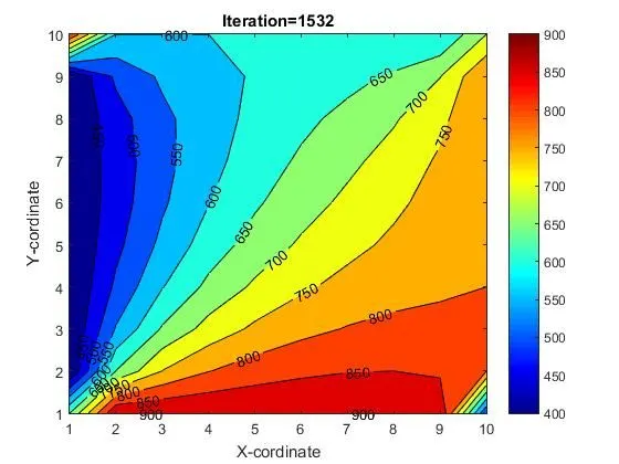
The number of iterations to get converged solution is 1532.
iii . Succesive over-relaxation Method:
The discritized eqaution using Succesive over-relaxation Method is:
`Toverset(n+1) i,j` = `(1-w) Told overset(n) i,j` + `w ( `Told(i,j) (1-2k1-2k2) + ((T(i-1,j) + Told(i+1,j) )k1 +(T(i,j-1) + Told(i,j+1)) k2 ) )``
Plot shows temperature distribution using Succesive over-relaxation iterative solver technique.
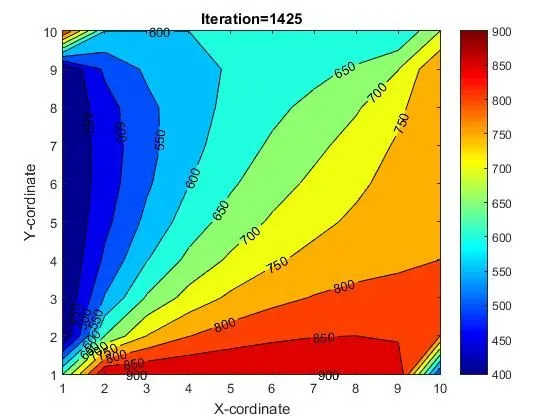
The number of iterations to get converged solution is 1425 for over-relaxation factor of 1.5.
II. Implicit Scheme:
Formulating implicit sheme requires more involved procedure as compared to explicit scheme, as this contains the terms whose values are unknown. This structure gives a scheme the inherent stability irrespective of the time step value used. That is why fewer time steps are needed to carry out calclation over a given interval. But this is not suitable for time accurate solution i.e exact transient may not be captured accurately, gives good results when steady state answer is desired.
1. Formulation:
The unsteady hat conduction equation in implicit form is:
`Toverset(n+1) i,j` = ``Tprev(i,j) k3 +`(Told(i-1,j) + Told(i+1,j)) overset (n) k1*k3`+`(Told(i,j-1) + Told(i,j+1)) overset (n) k2*k3`
where subscript 'i' and 'j' represents the location of respctive node.
2. Program:
MATLAB code is used to solve 2D unsteady heat conduction equation using implicit scheme.
clear all
close all
clc

% Defining Mesh
m =10;
n =10;
L=1;
dx=L/(m-1);
dy=L/(n-1);

% Initialising
% Boundary Conditions

T=20*ones(m,n); % Defining initial temp at all grid points
T(1,:)=900;
T(m,:)=600;
T(:,1)=400;
T(:,n)=800;
T(1,1)=650;
T(1,n)=500;
T(m,n)=700;
T(m,1)=850;
Told=T;
Tprev=T;

% Defining constants and variables

dt=0.1;
t=100;
nt=t/dt;

%alpha=20.34e-6 % alpha=k/pc (m^2/sec) thermal diffusivity, for pure iron block at 20 degree celcius, density=7897kgper m^3,specific heat=452 j/kgK, thermal conductivity k=72.7 w/mk

alpha=1e-2           %Reducing alpha increases computational time.
k1=(alpha*dt)/dx^2;
k2=(alpha*dt)/dy^2;
k3=1/(1+2*k1+2*k2);
tol=1e-4;


%% ________________________________________________________________________________

iterative_solver=3


%% ________________________________________________________________________________

% Jacobi Method

if iterative_solver==1
   jac_iter=1 % Itereration counter variable

 %Time loop
 for k=1:nt

     error=9e9;


    %Convergence Loop

    while(error>tol)

        %space loop

        for i=2:m-1

            for j= 2:n-1

                  T(i,j)= k3*(Tprev(i,j)+(Told(i-1,j)+Told(i+1,j))*k1 + (Told(i,j-1)+Told(i,j+1))*k2);
            end

        end

            error = max(max(abs(T-Told)))
            Told=T;            % Updating values of Told for next iteration
            jac_iter=jac_iter+1


 end

    Tprev=T; % Updating values of Tprev for next time step

 end

% Plotting results
%Results shopuld be plotted outside convergence loop to capture converged results

 figure(1)
 contourf(T,'ShowText','ON')
 colorbar;
 colormap(jet);
  xlabel('X-cordinate');
 ylabel('Y-cordinate');
 title_x=sprintf('Iteration=%d',jac_iter)
 title(title_x)
 pause(0.01);
end


%% ____________________________________________________________________________________

% Gauss-seidel Method

if iterative_solver==2
  gs_iter=1;

  % Time loop

   for k=1:nt
    error=9e9;

    % Convergence Loop

    while(error>tol)

        %Space Loop

        for i=2:m-1
            for j= 2:n-1
                  T(i,j)= k3*(Tprev(i,j)+(T(i-1,j)+Told(i+1,j))*k1 + (T(i,j-1)+Told(i,j+1))*k2);
            end
        end
            error = max(max(abs(T-Told)));
            Told=T;               % Updating values of Told for next iteration
            gs_iter=gs_iter+1;
    end

    Tprev=T;                      % Updating values of Tprev for next time step

   end

 % Plotting
 %Results shopuld be plotted outside convergence loop to capture converged results

 figure(2)
 contourf(T,'ShowText','ON')
 colorbar;
 colormap(jet);
 xlabel('X-cordinate');
 ylabel('Y-cordinate');
 title_x=sprintf('Iteration=%d',gs_iter)
 title(title_x)
end


%% _________________________________________________________________________________

% Succesive Over-Relaxation Method

if iterative_solver==3
  sor_iter=1;

  %Time loop

   for k=1:nt
    error=9e9;
    w=1.1;

    % Convergence Loop

    while(error>tol)

        %Space Loop

        for i=2:m-1
            for j= 2:n-1
                  T(i,j)= (1-w)*Told(i,j) + w*(k3*(Tprev(i,j)+(T(i-1,j)+Told(i+1,j))*k1 + (T(i,j-1)+Told(i,j+1))*k2));
            end
        end
            error = max(max(abs(T-Told)));
            Told=T;
            sor_iter=sor_iter+1;

    end
    Tprev=T;
   end

%Plotting
%Results shopuld be plotted outside convergence loop to capture converged results

 figure(3)
 contourf(T,'ShowText','ON')
 colorbar;
 colormap(jet);
 xlabel('X-cordinate');
 ylabel('Y-cordinate');
 title_x=sprintf('Iteration=%d',sor_iter)
 title(title_x)
end
3. Results:
i . Jacobi Method:
The discritized eqaution using Jacobi Method is:
`Toverset(n+1) i,j`= `Tprev(i,j) k3 +`(Told(i-1,j) + Told(i+1,j)) overset (n) k1*k3`+`(Told(i,j-1) + Told(i,j+1)) overset (n) k2*k3`
Here, old values are used everywhere for a given iteration.
Plot shows temperature distribution using Jacobi iterative solver technique.
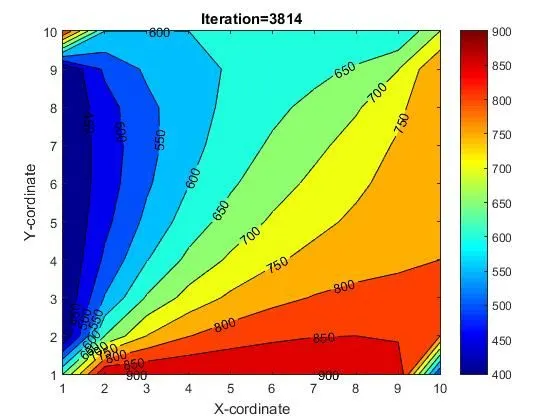
The number of iterations to get converged solution is 3814.
ii . Gauss-seidel Method:
The discritized eqaution using Gauiss-seidel Method is:
`Toverset(n+1) i,j`=``Tprev(i,j) k3 +`(T(i-1,j) + Told(i+1,j)) overset (n) k1*k3`+`(T(i,j-1) + Told(i,j+1)) overset (n) k2*k3`
Here, updated values are used i.e Told is replaced by T as the new temperature values are being calculated in previous iteration.
Plot shows temperature distribution using Gauss-seidel iterative solver technique.
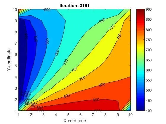
The number of iterations to get converged solution is 3191.
iii . Succesive over-relaxation Method:
The discritized eqaution using Succesive over relaxation Method is:
`Toverset(n+1) i,j`= `(1-w) Told overset (n+1) i,j` + w k3 (`Tprev(i,j) k3 + `(T (i-1,j) + Told (i+1,j) )overset (n)` k1 + `(T (i,j-1) + Told (i,j+1) ) overset (n) ` k2`
Plot shows temperature distribution using Succesive over-relaxation iterative solver technique.
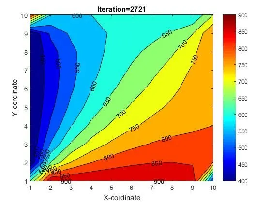
The number of iterations to get converged solution is 2721 for over-relaxation factor of 1.1
Conclusion:
The steady as well as unsteady 2D heat conduction equation are being soved using three iterative technique in Explicit and implicit form.
It is observed that,
1. Gauss-seidel iterative method converges faster as compared Jacobi Iterative method as it uses the updated values calculated in previous iteration.
2. Succeive over-relaxation Method happens to be converging more aggresively than Jacobi and Gauss-seidel method due to high relaxation factor used in method.