Week 7 - Simulation of a 1D Super-sonic nozzle flow simulation using Macormack Method
Aim:
To simulate the isentropic flow through a quasi 1D subsonic-supersonic nozzle using the MacCormack's technique for both conservation and non-conservation forms of the governing equations.
Solution:
1. Important aspcts of compressible flow:
The flow through converging -diverging nozzle is compresible flow with fluid used as air. The important parameter use to study compressible flows is Sonic Speed (C).
C = `sqrt((dp)/(drho))`
'C' is an important property which relate to elasticity of medium which shows effect of compressibility directly. C inversly relate to what is rate of change of density with change in pressure. If very high 'dp' is required to create small change in desnsity then system becomes very hard to compress, ,more the compact system is higher and higher is C. So for such systems C becomes infinitely large that is why in in-compressible system the disturbance in form of pressure purturbations travels at infinite speed unlike not very compact compressible systems where finite C exist i.e Compreesible medium is like an elastic body.
'dp' and 'd`rho`' depends on the thermodynamic proces by which it is happening. In absence of any extyernal work and heat transfer to system, the process by which changes in pressure and density are achieved mostly is a reversible and adiabatic in nature i.e an Isentropic process. For a reversible adiabatic process the change in entropy is zero, which gives a expression for C.
`C = sqrt(gamma R T)`
where , R is Specific Gas Constant ( air = 287 j/kg.k ) T is absolutr temperature.
When flow takes place through nozzle the disturbance which can be characterized by pressure purturbations (weak pressure waves) is created (due to flow) in the elastic medium i.e compressible medium which is moving with velocity of 'C' and considering the flow itself is the source of disturbance the flow is moving at velocity of 'u'. The velocity with which disturbance and source moves is related by a dimensionless number called 'Mach number' (M).
`M = u / C`
For an isentropic process of an ideal gas,
`P/rho^gamma` = constant , with `gamma = (cp)/(cv)`
For an ideal gas 'cp' and 'cv' are not constant i.e are functions of temperature. But in the analysis we are using a special type of ideal gas which wil have constant cp and cv called as Calorically Perfect gas.
In case of high speed flows like flow through nozzle, the contribution of kinetic energy in the total energy of a system can not be neglected. The static entalpy and kinetic energy of system are combined together in a single term called as stagnation (total) enthalpy (h0) indicates total energy of flowing fluid per unit mass.In analysis of control volume the kinetic energy term is also included in steady flow energy equation (E in = E out).
`h1 + (V1^2)/2 = h2 + (V2^2)/2`
when fluid is brought to rest
`h1 + (V1^2)/2 = h2 = h02`
During stagnation process the fluid is brought to rest adiabatically and kinetic energy of fluid is converted into enthaly which results in increase in temperature and pressure of fluid . The properties at stagnation state are called stagnation properties. These properties dictate the nature of process by which stagnation is achieved.
The general expresion to calculate stagnation temperature at a point is given by
`T0 = T + (u^2)/(2*cp)`
but when process is isentropic in nature then stagnation temperature and a static temperature at a point are related by
`(T0)/T = 1 + (gamma -1)/2 * M^2`
similarly for a pressure
`(P0)/P = ((T0)/T )^(gamma/gamma-1) = [1 + (gamma-1)/gamma * M^2 ]^(gamma/(gamma-1))`
i. Stagnation properties are used as reference properties, stagnation properties will exist for a point even if point is not a stagnation point because the expressions rae combination of proerties only.
ii. In order to achieve stagnation physically, flow need to be brought down to rest adiabatically without imposing condition of reversibility.
The purpose of nozzle is to accelerate the flow and the shape of nozzle governs this. For compressible flows converging geometry does not ensure that it is nozzle because density is also varying with time unlike in incompressible flows. It need to be decided from following expressions.
`(dA)/A = (M^2 -1)* (du)/u` `(dA)/A = (1-M^2)* (dp)/(rho u^2)`
From expressions,
When,
M<1 `rightarrow` Converging section (dA/A is decreasing) `rightarrow` velocity will increase , pressure will decrease.
M>1 `rightarrow` Diverging section (dA/A is increasing) `rightarrow` velocity will further increase and pressure will further decrease.
To accelerate fluid it is necessary to use converging nozzle at subsonic velocities and diverging nozzle at supersonic velocities.
dA/A = 0
when,
- M = 1 i.e at sonic condition, which means area attains a either a minimum or maximum value but from further expressions it can be conclude that dA/A = 0 gives a minumum area. That minimum area region is called 'Throat'.
- also at du/u =0, which concludes that at some area if M=1 is achieved then it is minimun area (throat), but minimum area will not ensure to have M=1. so M=1 can be at any area , but in this analysis m=1 is achieved at throat.
The properties at sonic condition can be used as a reference quantities given by `p^(star)`,`u^(star)`,`rho^(star)`,`A^(star)`. `A^(star)` is at some condition what should be the area at which sonic condition is achieved. So corresponding to each state there is corresponding starred quantities.
At given M , `p/(p0) , T/(T0),rho/(rho0),A/(A^(star))` can be caluclated and tabulated in data tables and that are used for calulations.
Governing equations:
The governing equationbs are as follows:
1. Conservative form:
Continuty Equation:
`(del(rhoA))/(delt) + (del(rhoAv))/(delt) = 0`
Momentum Equation:
`(del(rhoAv))/(delt) + (del(rhoAv^2))/(delx) = -( delp)/(delx`
Energy Equation:
`(del(rhoAv^2))/(delt) +(del(rhoAv^3))/(delx) = -Av(delp)/(delx)`
2. Non-conservation form
Continuty Equation:
`(del(rhoA))/(delt) + v *(del(rhoA))/(delx) + rhoA*(del(v))/(delx) = 0`
Momentum Equation:
`rho*(delv)/(delt) + rhoA *(delv)/(delx) = - (delp)/(delx`
Energy Equation:
`rho*(delrho)/(delt) + rhov *(delrho)/(delx) = -rho (delv)/(delx) - pv*(del(logA))/(delx)`
The above equations are non-dimensionalize using
`overlineT = T/(To) , overlinerho = rho/(rhoo) , overlinex = x/L , overlinet = t/(L/(Co)) , overlinev = v/(Co) , overlineA = A/A^(star)`
where, L = length of nozzle
Co = `sqrt(gammaRTo`
Final expression for Non-Conservative forms are:
`(delp)/(delt) = - rho*(delv)/(delx) - rhov(del(logA))/(delx) - v*(delrho)/(delx`
`(delv)/(delt) = v*(delv)/(delx) - (1/gamma* ((delT)/(delx) + T/rho * (delrho)/(delx)))`
`(delT)/(delt) = - v*(delT)/(delx) - (gamma-1)*T*((delv)/(delx) + v*(del(logA))/(delx))`
Here for convinience `overlineT , overlinerho ,overlinex, overlinet,overlinev,overlineA` are indicated by T,`rho`,x,t,v,A in non-dimensionalized governing equation further.
Numerical Domain:
Nozzle length is divided into 31 discrete points with node number 1 as inlet and node number 31 indicating outlet. The node number 16 is a throat i.e section with minimum area as shown in figure:
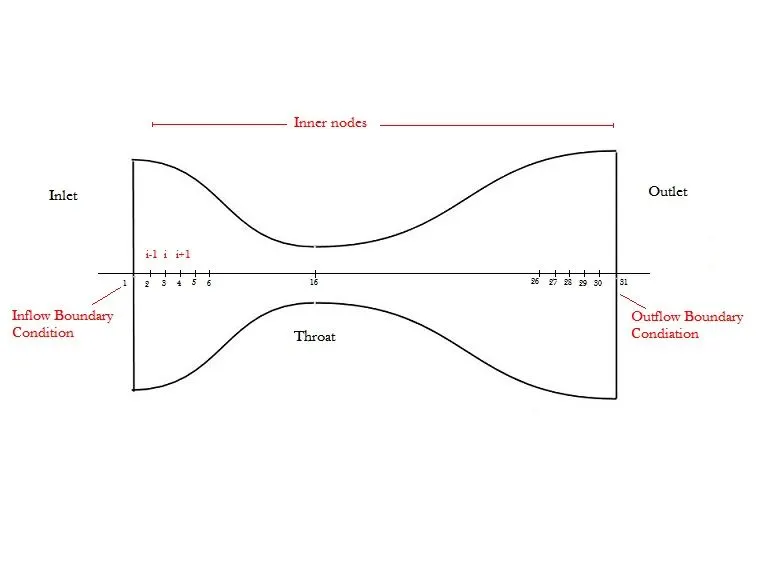
Figure 1: Numerical Domain
Numerical Technique:
Maccormack's technique is used to solve the governing equations of nozzle. Mccormack's technique is a Explicit finite difference technique of second order accurate both in space and time.The solution is obtained by time marching and value at t+dt is predicted on taylors series expansion in time.
`f overset(t+Deltat)` `= f oversett``+ ((delf)/(delt))overset(t)(avg)`
`((delf)/(delt) )overset (avg)` is calculated to maintain second order accuracy through a predictor and corrector steps: 'f' at t is calculated from initial conditions.
1. Predictor step:
Spatial derivatives in RHS will be discritised by forward differencing.
`((delrho)/(delt))overset(t)(p) =``( -rho (i) *((v(i+1)-v(1))/(Deltax)) - rho(i)*v(i)*((log(A) (i+1)-log(A)(i))/(Deltax)) - v(i)*((rho(i+1)-rho(i))/(Deltax)))oversett`
Now this value is use to get value at time step t i.e solution is updated for first time step.
`rho overset(t+Deltat)``= rho overset t``+ ((delrho)/(delt))overset(t)(p)`
2. Corrector step:
Spatial derivatives in RHS will be discritised by backward differencing.
`((delrho)/(delt))overset(t)(c) =``( -rho (i) *((v(i)-v(i-1))/(Deltax)) - rho(i)*v(i)*((log(A) (i)-log(A)(i-1))/(Deltax)) - v(i)*((rho(i)-rho(i-1))/(Deltax)))oversett`
3. Average Value:
`((delrho)/(delt))overset(t)(avg)`= 0.5 [`((delrho)/(delt))overset(t)(p)`+ `((delrho)/(delt))overset(t)(c)`]
This allows to obtain the final, "corrected" value of density at time t + dt as:
`rho overset(t+Deltat)``= rho oversett``+ ((delrho)/(delt))overset(t)(avg)`
This sequence is repeated at all grid point's to obtain the density throughout the flow field at time t + dt. To calculate v,T at t + dt the same technique is used.
Time step calculation:
The governing equations are hyperbolic with respect to time and their stability is constrained by the value of time increment in marching dirction. If the `Deltat` is greater than a critical value then solution will be likely to go unstable. The value of courant number ensures the stability. In this problem value of courant number is taken as 0.5 so the `Deltat`is given by
`Deltat = (C*Deltax)/((c+v))`
where C=0.5 and (c+v) is the combined velocity of flow and disturbance as both are moving in same direction.
`Deltat` = minimum ( `Deltatunderset1`,`Deltatunderset2`,`Deltatunderset3`,.......,`Deltatundersetn`)
The minimum value out of all values corresponding to each location is the `Deltat` used for the actual calculation which is found to be 0.0216.
Initial Condition:
To start the time-marching calculations it is important to set up values of p, T, v at time t=0 and is done by initial conditions as given below.
`rho = 1 -0.346*x`
`Y = 1- 0.2314*x`
`v = (0.1 + 1.09*x)*T^0.5`
`A = 1 + 2.2*(x-1.5)^2`
Boundary Conditions:
The unsteady - inviscid flow is governed by hyperbolic equation eg. 1D wave equation ;
`(del^2phi)/(delt^2) = c^2 * (del^2phi)/(delx^2)`
This equation have two characteristics whoch shows that effect is not a function of time only or space only but it is a spacio-temporal effect. For this one dimensional unsteady equation there are two real characteristic lines x+ct and x-ct exist which represent two weak Mach waves travelling at speed of sound c.
At subsonic inflow the one characteristic line flows in and another out. From method of characteristics tells that when one characteristic line propgete into then one dependent flow field variable must be specified at inlet boundary, we specify values of density and temperature at inlet i.e at reservoir where flow velocity is considered very small so these values become equals to stagnation values at inlet.Another characteristic line flows out which states that value of second dpendent variable must be allowed to float i.e must be evaluated in steps of time as function of timewise solution of flow field. Here we are allowing value of velocity to float, Physically it is natural that mass flow will be going to adjust to a steady stte value so 'v' is llowed to float.
Value of v changes with time and is calculated from information provided by flow field solution over internal points. That is why value at point 1 is calculated by linear extrapolation from point 2 and 3
v1 = v2 - slope
v1 = v2 - `(v3-v2)/(Deltax)` `Deltax` = v1 = 2v2 - v3
and density and temperature are known i.e stagnation values.
At Supersonic outflow, both characteristics flows outwards so all variableas need to be caluclated over the period of time. The values are calculated using linear extrapolation:
v(n) = 2 v(n-1) - v(n-2)
`rho(n) = 2 rho(n-1)-rho(n-2)`
T(n) = 2 T(n-1) - T(n-2)
The values of flow variable at outlet is depend on corresponding values at n-1 and n-2 but not a vice-versa that is why it is a neumann type of boundry condition.
Program:
a) Non-conservative form:
The following MATLAB program is used to solve governing equation in non- conservative form.
clc
close all
clear all

% grid
n  = 31;
x  = linspace(0,3,n);
dx = x(2)-x(1);

%initial Condition
rho = 1-0.3146*x;
T   = 1-0.2314*x;
v   = (0.1 + 1.09*x).*T.^0.5
A   = 1+2.2*(x-1.5).^2;
gamma = 1.4;

% Time steps
C  = 0.5;
nt = 1000;
dt = min((C*dx)./(sqrt(T)+v));
throat = 16; %16th node


% outer Time loop

for k = 1:nt

    % predictor step
    rho_old = rho;
    v_old   = v;
    T_old   = T ;

    for i = 2:n-1

    % d_rho_dt = - rho(i)*((v(i+1)-v(i))/dx) - (rho(i)*v(i)*((log(a(i+1))-log(a(i)))/dx)) - v(i)*((rho(i+1)-rho(i))/dx)

    dvdx      = ((v(i+1)-v(i))/dx);
    dlog_A_dx = (log(A(i+1))-log(A(i)))/dx;
    drhodx    = (rho(i+1)-rho(i))/dx;
    dTdx      = (T(i+1)-T(i))/dx;

    % Continuty equation
drhodt_p(i) = - rho(i)*dvdx - (rho(i)*v(i)* dlog_A_dx) - (v(i)*drhodx) ;

    % Momentum equation
dvdt_p(i)   = - v(i)*dvdx - (1/gamma)*(dTdx + (T(i)/rho(i))* drhodx);

    % Energy equation
dTdt_p(i)   = - v(i)*dTdx - ((gamma-1)*T(i)*(dvdx + v(i)*dlog_A_dx));


    % Solution update

rho(i) = rho(i) + drhodt_p(i) * dt;
v(i)   = v(i) + dvdt_p(i) * dt;
T(i)   = T(i) + dTdt_p(i) * dt;

    end

    for i= 2:n-1

 % Corrector step

    dvdx      = ((v(i)-v(i-1))/dx);
    dlog_A_dx = (log(A(i))-log(A(i-1)))/dx;
    drhodx    = (rho(i)-rho(i-1))/dx;
    dTdx      = (T(i)-T(i-1))/dx;


    % Continuty equation

    drhodt_c(i) = - rho(i)*dvdx - (rho(i)*v(i)* dlog_A_dx) - (v(i)*drhodx) ;

    % Momentum equation

    dvdt_c(i)   = - v(i)*dvdx - (1/gamma)*(dTdx + (T(i)/rho(i))* drhodx);

    % Energy equation

    dTdt_c(i)   = - v(i)*dTdx - ((gamma-1)*T(i)*(dvdx + v(i)*dlog_A_dx));

    end

 % Calculating new time derivative called Average Time Derivative

 drhodt_avg = 0.5 * (drhodt_p + drhodt_c);
 dvdt_avg   = 0.5 * (dvdt_p + dvdt_c) ;
 dTdt_avg   = 0.5 * (dTdt_p + dTdt_c) ;

 % Computing actual values of variable in second time step i.e final solution update

 for j = 2:n-1

     rho(j) = rho_old(j) + drhodt_avg(j) * dt
     v(j)   = v_old(j) + dvdt_avg(j) * dt
     T(j)   = T_old(j) + dTdt_avg(j) * dt

 end


% Applying Boundary conditions

% Inflow boundary condition

  v(1) = 2* v(2) - v(3) ;

% Outflow Boundary Condition

  rho(n) = 2*rho(n-1) - rho(n-2);
  v(n)   = 2* v(n-1) - v(n-2);
  T(n)   = 2* T(n-1) - T(n-2);


  % Mach number
   M = v./sqrt(T);
   % mass flow rate
   m = rho.*A.*v;
   P   = rho.* T;
   % Throat values for transient plots
   rho_throat(k) = rho(throat);
   v_throat(k) = v(throat);
   T_throat(k) = T(throat);
   P_throat(k) = P(throat);
   M_throat(k) = M(throat);

   % Transient mass flow rate plots
   figure(1)
   if k == 1
     plot(x,m)
     hold on
   end
   if k == 100
     plot(x,m)
   end
   if k == 300
     plot(x,m)
   end
   if k == 700
     plot(x,m)
   end
   if k == 1000
     plot(x,m)
   end
   if k == 1400
     plot(x,m)
   end

end

%Figure(1) plot details
ylabel('mass flow rate')
xlabel('Timestep')
title('Variation of mass flow rate at different time steps')
legend('1dt','100dt','300dt','700dt','1000dt')


figure(2)

subplot(2,2,1)
plot(x,rho)
xlabel('x/L')
ylabel('rho/rho0')
title('Steady state profiles of primitive variables across the nozzle')
grid on
subplot(2,2,2)
plot(x,M)
xlabel('x/L')
ylabel('Mach Number')
grid on
subplot(2,2,3)
plot(x,T)
xlabel('x/L')
ylabel('T/T0')
grid on
subplot(2,2,4)
plot(x,P)
xlabel('x/L')
ylabel('P/P0')
grid on

figure(3)
subplot(2,2,1)
plot(rho_throat)
xlabel('x/L')
ylabel('rho/rho0')
title('Transient profiles of primitive variables at throat')
subplot(2,2,2)
plot(M_throat)
xlabel('x/L')
ylabel('Mach no')
subplot(2,2,3)
plot(T_throat)
xlabel('x/L')
ylabel('T/T0')
subplot(2,2,4)
plot(P_throat)
xlabel('x/L')
ylabel('P/P0')
Output:
The output of the program is given below,
|
Final values of all variables for non conservative form |
||||||
|
x/L |
A/A˳ | P/P˳ | ρ/ρ˳ | T/T˳ | v/C˳ | m/m˳ |
| 0.1 | 5.312 | 0.996915 | 0.997799 | 0.999114 | 0.112009 | 0.593682 |
| 0.2 | 4.718 | 0.995844 | 0.99703 | 0.998811 | 0.125231 | 0.589085 |
| 0.3 | 4.168 | 0.991986 | 0.994271 | 0.997702 | 0.142617 | 0.591024 |
| 0.4 | 3.662 | 0.988325 | 0.991646 | 0.996651 | 0.162266 | 0.589254 |
| 0.5 | 3.2 | 0.982312 | 0.987333 | 0.994914 | 0.186561 | 0.589435 |
| 0.6 | 2.782 | 0.97463 | 0.98181 | 0.992686 | 0.215446 | 0.588469 |
| 0.7 | 2.408 | 0.963485 | 0.973777 | 0.989431 | 0.250775 | 0.588032 |
| 0.8 | 2.078 | 0.948064 | 0.962614 | 0.984885 | 0.293577 | 0.587246 |
| 0.9 | 1.792 | 0.926142 | 0.946655 | 0.978332 | 0.345789 | 0.586599 |
| 1 | 1.55 | 0.895445 | 0.924119 | 0.968972 | 0.409028 | 0.585885 |
| 1.1 | 1.352 | 0.85286 | 0.89248 | 0.955607 | 0.48504 | 0.585265 |
| 1.2 | 1.198 | 0.795539 | 0.849157 | 0.936857 | 0.574778 | 0.584716 |
| 1.3 | 1.088 | 0.721761 | 0.792047 | 0.91126 | 0.678018 | 0.58428 |
| 1.4 | 1.022 | 0.632844 | 0.720946 | 0.877797 | 0.792537 | 0.583946 |
| 1.5 | 1 | 0.534203 | 0.638658 | 0.836446 | 0.914018 | 0.583745 |
| 1.6 | 1.022 | 0.434509 | 0.550994 | 0.788591 | 1.036658 | 0.583759 |
| 1.7 | 1.088 | 0.342571 | 0.464951 | 0.73679 | 1.15461 | 0.584078 |
| 1.8 | 1.198 | 0.264248 | 0.386322 | 0.68401 | 1.263403 | 0.58472 |
| 1.9 | 1.352 | 0.20146 | 0.318352 | 0.632822 | 1.360579 | 0.585609 |
| 2 | 1.55 | 0.153145 | 0.261813 | 0.584938 | 1.445571 | 0.586628 |
| 2.1 | 1.792 | 0.116858 | 0.215901 | 0.541256 | 1.518951 | 0.587674 |
| 2.2 | 2.078 | 0.089884 | 0.179059 | 0.501983 | 1.582064 | 0.58866 |
| 2.3 | 2.408 | 0.069886 | 0.149643 | 0.467014 | 1.636167 | 0.589579 |
| 2.4 | 2.782 | 0.054964 | 0.12609 | 0.435915 | 1.682939 | 0.590345 |
| 2.5 | 3.2 | 0.043782 | 0.107205 | 0.408395 | 1.72309 | 0.591116 |
| 2.6 | 3.662 | 0.035254 | 0.091857 | 0.383794 | 1.758557 | 0.591541 |
| 2.7 | 4.168 | 0.028778 | 0.079475 | 0.362104 | 1.788663 | 0.592495 |
| 2.8 | 4.718 | 0.023631 | 0.069041 | 0.342275 | 1.816707 | 0.591763 |
| 2.9 | 5.312 | 0.019827 | 0.060953 | 0.325279 | 1.839244 | 0.595515 |
| 3 | 5.95 | 0.016298 | 0.052866 | 0.308282 | 1.86178 | 0.585623 |
Formulation of Conservative Form :
Non dimensionalized Conservation form :
Continuty equation:
`(del(rho*A))/(delt) + (del(rho*A*v))/(delx) = 0`
Momentum Equation:
`(del(rho*A*v))/(delt) + (del(rho*A*v^2 + (1/gamma)*p*A))/(delx) = 1/gamma *p*(delA)/(delx)`
Energy Equation:
`(del((e/(gamma-1) + (gamma/2)*v^2)*A))/(delt) + (del((rho*(e/(gamma-1) + (gamma/2)*v^2)*v*A)+rho*A*v))/(delx) = 0`
Conservative form of governing equations provides numerical and computer convenience that the complex governing equations can be expressed in form of some generic equations. These generic equations are formed by dividing main governing equation in form of Flux terms, Source terms and solution terms.
Left side of all governing equations do contain a divergence terms, which involves divergence of the flux of some physical quantities
i.e for Continuty equation : `rho*v` mass flux
for x momentum equation : `rho*u*V` Flux of x component of momentum
for energy equation : `rho*V*(e+v^2/2)` Flux of total energy
Solution vector is set of terms which are dependent variables which are calculated numerically in steps of time.
Column vector F, G, H are called 'Flux vector'.
Column vector J is called 'Source vector'.
Column vector U us called 'Solution vector'.
The equivalent same generic form is:
`(delU)/(delt) + (delF)/(delx) + (delG)/(dely) + (delH)/(delz) = J`.
`(delU)/(delt) = J - (delF)/(delx) - (delG)/(dely) - (delH)/(delz)`
Spatial dervatives on right side are considered in some respect are known i.e. from the previous time step. Variables such as P,v,`rho` are called primitive variables.
For given equation:
U1 = `rho*A`
U2 = `rho*A*v`
U3 = `rho*((e/(gamma-1) + gamma/2*v^2)*A)`
F1 = `rho*A*v`
F2 = `rho*A*v + 1/gamma * p*A`
F3 = `rho*(e/(gamma-1) + gamma/2*v^2)*v*A + rho*A*v`
J2 = `1/gamma *p*(delA)/(delx)`
Now the generic equations that are to be solved in program are:
`(delU1)/(delt) = - (delF1)/(delx)`
`(delU2)/(delt) = - (delF2)/(delx) + J2`
`(delU3)/(delt) = - (delF3)/(delx)`
here, F1,F2,F3and J2 are formulated in form of U1,U2,U3. In conservation form dependent variables are not primtive variables. So solution will give values of primitives variables. i.e. primitive variables like p,v`rho` are caluclated from values of U1,U2,U3.
`rho = (U1)/(A1`
`v = (U2)/(U1`
`T = e = (gamma-1) * ((U3)/(U1)- (gamma/2)*v^2)`
`p = rho*T`
U1, U2, U3 are calculated for each time step and respective primitive variabls are calculated at each time step. This equations are solved using Maccormack technique using corrector-prdictor methodology which can be sen in following program.
Program:
b) Conservative Form
MATLAB code is used to solve governing equation in conservation form:
close all
clear all
clc

% grid
n  = 31;
x  = linspace(0,3,n);
dx = x(2)-x(1);

%initial profiles
A   = 1+2.2*(x-1.5).^2;
rho = 1-0.3146*x;
T   = 1-0.2314*x;
v   = 0.59./(rho.*A);

gamma = 1.4;

%initial conditions for generic forms variables

e = T ;
U1 = rho .* A;
U2 = rho .* v .* A;
U3 = rho .* A .* ((T/(gamma-1)) + (gamma/2) * v.^2);

% Time steps
C  = 0.5;
nt = 1400;
dt = min((C*dx)./(sqrt(T)+v));
throat = 16; %16th node


% time loop
for k = 1:nt

   U1_old = U1 ;
   U2_old = U2 ;
   U3_old = U3 ;

   % Flux Terms

   F1 = U2 ;
   F2 = ((U2.^2)./U1) + ((gamma-1)/gamma)*(U3 - ((gamma/2)*((U2.^2)./U1))) ;
   F3 = gamma * ((U2.*U3)./U1) - ((gamma * (gamma-1)/2) * ((U2.^3)/U1.^2));

   % calling function to solve for u1,U2,U3.
   for i =2:n-1


   dF1_dx = (F1(i+1)-F1(i))/dx ;
   dF2_dx = (F2(i+1) - F2(i))/ dx ;
   dF3_dx = (F3(i+1) -F3(i))/dx ;
   dAdx   = (A(i+1) - A(i))/dx ;
   J2     = ((dAdx) .* rho(i) .* T(i))/gamma;


   dU1_dt_p(i) = - dF1_dx ;
   dU2_dt_p(i) = - dF2_dx + J2 ;
   dU3_dt_p(i) = - dF3_dx ;

   % updating (finding) values of U

   U1(i) = U1(i) + dU1_dt_p(i)*dt ;
   U2(i) = U2(i) + dU2_dt_p(i)*dt ;
   U3(i) = U3(i) + dU3_dt_p(i)*dt ;

   end

   % calculating new values of primitive variables from updated (new) valeus of U1,U2,U3

   rho = U1./A ;
   v   = U2./U1 ;
   T   = (gamma-1)* ( (U3./U1) - ((gamma/2)* v.^2) );
   P   = rho.* T;

   % caluclating new F

   F1 = U2 ;
   F2 = (U2.^2./U1) + ((gamma-1)/gamma)*(U3 - ((gamma/2)*(U2.^2./U1))) ;
   F3 = gamma * (U2.*U3./U1) - ((gamma * (gamma-1)/2) * (U2.^3/U1.^2)) ;

   % Corrector method

   for i = 2:n-1


   dF1_dx = (F1(i)-F1(i-1))/dx ;
   dF2_dx = (F2(i) - F2(i-1))/ dx ;
   dF3_dx = (F3(i) -F3(i-1))/dx ;
   dAdx   = (A(i) - A(i-1))/dx ;
   J2     = ((dAdx) .* rho .* T)/gamma;


   dU1_dt_c(i) = - dF1_dx ;
   dU2_dt_c(i)  = - dF2_dx + J2(i) ;
   dU3_dt_c(i)    = - dF3_dx ;

   end

   % average values

   dU1_dt_avg = 0.5* ( dU1_dt_p + dU1_dt_c ) ;
   dU2_dt_avg = 0.5* ( dU2_dt_p + dU2_dt_c ) ;
   dU3_dt_avg = 0.5* ( dU3_dt_p + dU3_dt_c ) ;

  % new values of U
  for j =2:n-1

  U1(j) = U1_old(j) + dU1_dt_avg(j)*dt;
  U2(j) = U2_old(j) + dU2_dt_avg(j)*dt;
  U3(j) = U3_old(j) + dU3_dt_avg(j)*dt;

  end

  % aplying B.C

  % inlet
   U1(1) = rho(1)* A(1) ;
   U2(1) = 2* U2(2) - U2(3) ;
   v(1)  = U2(1)/U1(1) ;
   U3(1) = rho(1)*A(1)* ((T(1)/(gamma-1)) + ((gamma/2)*v(1)^2)) ;

   % Outlet

   U1(n) = 2* U1(n-1) - U1(n-2) ;
   U2(n) = 2* U2(n-1) - U2(n-2) ;
   U3(n) = 2* U3(n-1) - U3(n-2) ;

   % Calculating final alue of primitive variables


   rho = U1./A ;
   v   = U2./U1 ;
   T   = (gamma-1)* ( (U3./U1) - ((gamma/2)* v.^2) ) ;
   P   = rho.* T ;
   % Mach number
   M = v./sqrt(T);
   % mass flow rate
   m = rho.*A.*v;


   % Throat values for transient plots
   rho_throat(k) = rho(throat);
   v_throat(k) = v(throat);
   T_throat(k) = T(throat);
   P_throat(k) = P(throat);
   M_throat(k) = M(throat);


   % Transient mass flow rate plots
   figure(1)
   if k == 1
     plot(x,m)
     hold on
   end
   if k == 100
     plot(x,m)
   end
   if k == 300
     plot(x,m)
   end
   if k == 700
     plot(x,m)
   end
   if k == 1000
     plot(x,m)
   end
   if k == 1400
     plot(x,m)
   end

end
%Figure(1) plot details
ylabel('mass flow rate')
xlabel('Timestep')
title('Variation of mass flow rate at different time steps')
legend('1dt','100dt','300dt','700dt','1000dt','1400dt')


figure(2)

subplot(2,2,1)
plot(x,rho)
xlabel('x/L')
ylabel('rho/rho0')
title('Steady state profiles of primitive variables across the nozzle')
grid on
subplot(2,2,2)
plot(x,M)
xlabel('x/L')
ylabel('Mach Number')
grid on
subplot(2,2,3)
plot(x,T)
xlabel('x/L')
ylabel('T/T0')
grid on
subplot(2,2,4)
plot(x,P)
xlabel('x/L')
ylabel('P/P0')
grid on

figure(3)
subplot(2,2,1)
plot(rho_throat)
xlabel('x/L')
ylabel('rho/rho0')
title('Transient profiles of primitive variables at throat')
subplot(2,2,2)
plot(M_throat)
xlabel('x/L')
ylabel('Mach no')
subplot(2,2,3)
plot(T_throat)
xlabel('x/L')
ylabel('T/T0')
subplot(2,2,4)
plot(P_throat)
xlabel('x/L')
ylabel('P/P0')
Output:
The output of the program is given below,
|
Final values of all variables for non conservative form |
|
x/L |
A/A˳ | P/P˳ | ρ/ρ˳ | T/T˳ | v/C˳ | m/m˳ |
| 0.1 | 5.312 | 0.998038 | 0.998813 | 0.999224 | 0.117145 | 0.621536 |
| 0.2 | 4.718 | 0.995416 | 0.997243 | 0.998168 | 0.132112 | 0.621587 |
| 0.3 | 4.168 | 0.991925 | 0.995131 | 0.996778 | 0.149859 | 0.62157 |
| 0.4 | 3.662 | 0.987171 | 0.99227 | 0.994861 | 0.17107 | 0.621614 |
| 0.5 | 3.2 | 0.980666 | 0.988326 | 0.992249 | 0.19655 | 0.621616 |
| 0.6 | 2.782 | 0.97163 | 0.982852 | 0.988582 | 0.227358 | 0.621664 |
| 0.7 | 2.408 | 0.958996 | 0.975144 | 0.98344 | 0.264755 | 0.621685 |
| 0.8 | 2.078 | 0.941191 | 0.964241 | 0.976095 | 0.3103 | 0.621746 |
| 0.9 | 1.792 | 0.916099 | 0.94872 | 0.965616 | 0.365732 | 0.621783 |
| 1 | 1.55 | 0.880926 | 0.926728 | 0.950577 | 0.432918 | 0.621855 |
| 1.1 | 1.352 | 0.832516 | 0.89589 | 0.929261 | 0.513425 | 0.621883 |
| 1.2 | 1.198 | 0.767963 | 0.853746 | 0.899522 | 0.608067 | 0.621924 |
| 1.3 | 1.088 | 0.686242 | 0.798364 | 0.85956 | 0.715911 | 0.621855 |
| 1.4 | 1.022 | 0.589641 | 0.729496 | 0.808286 | 0.833996 | 0.621781 |
| 1.5 | 1 | 0.495528 | 0.657922 | 0.753172 | 0.944695 | 0.621535 |
| 1.6 | 1.022 | 0.384406 | 0.565654 | 0.679578 | 1.074838 | 0.621362 |
| 1.7 | 1.088 | 0.29323 | 0.481383 | 0.609141 | 1.186107 | 0.621217 |
| 1.8 | 1.198 | 0.218222 | 0.40352 | 0.540797 | 1.284899 | 0.621142 |
| 1.9 | 1.352 | 0.160202 | 0.335385 | 0.477666 | 1.36983 | 0.621137 |
| 2 | 1.55 | 0.117162 | 0.278039 | 0.421387 | 1.441339 | 0.621161 |
| 2.1 | 1.792 | 0.08601 | 0.230979 | 0.372371 | 1.50083 | 0.621215 |
| 2.2 | 2.078 | 0.06369 | 0.192861 | 0.33024 | 1.55016 | 0.621249 |
| 2.3 | 2.408 | 0.047726 | 0.162173 | 0.29429 | 1.591015 | 0.621313 |
| 2.4 | 2.782 | 0.036226 | 0.137427 | 0.2636 | 1.625121 | 0.621318 |
| 2.5 | 3.2 | 0.02789 | 0.117437 | 0.237489 | 1.653528 | 0.621395 |
| 2.6 | 3.662 | 0.021737 | 0.101133 | 0.214937 | 1.677746 | 0.621351 |
| 2.7 | 4.168 | 0.017202 | 0.087818 | 0.195878 | 1.697868 | 0.621462 |
| 2.8 | 4.718 | 0.013718 | 0.076757 | 0.178727 | 1.715842 | 0.621371 |
| 2.9 | 5.312 | 0.011158 | 0.067623 | 0.165004 | 1.730065 | 0.621463 |
| 3 | 5.95 | 0.009038 | 0.059881 | 0.15094 | 1.744521 | 0.621555 |
2. Results:
1. Non conservative form:
In order to set flow across nozzle always driving force is needed, that force arise in case of nozzle is due to the difference in pressure across nozzle inlet and outlet. Desired exit condition is not our choice but desired pressure in the chamber is in our control. That desired pressure in the chamber where nozzle exit is taking place is the Back pressure. Once flow is set whether it accelerate or decelerate depends on the set value of back pressure. In this problem the back pressure is same as that of exit pressure. In time marching approach we are solving for these variables considering some suitable initial condition result of which we get the pressure distribution across the length of nozzle as shown in figure. Non-dimensionalized value of pressure at exit (pe/po) is 0.0163. This indicates, as if we have maintained the non-dimensional back pressure (pb/po) to 0.0163. Due to this differential we will get the changes in density , velocity and temperature across nozzle inlet and outlet as shown in figure 2.
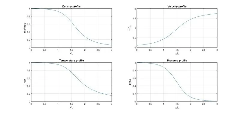
Figure 2: Variation of primitive variables
As pressure decreases the flow starts to accelerate i.e velocity is set in, and it keep on increasing as pressure goes down across the nozzle. The velocity at throat i.e at x/L = 1.5, it attains a sonic value and in diverging section it keep on increasing to accelerate flow further. Working fluid here is assumed to be a perfect gas so, as pressure reduces the density of fluid starts to decrease. In absence of any heat transfer, heat generation and friction inside nozzle the temperature will also decrease as flow proceeds. This behavior is as shown in figure 3 above,
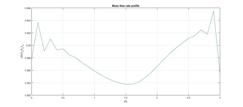
Figure 4: Mass flow rate profile across the one-dimensional Nozzle length
Figure 4, shows the mass flow rate variation across the length of nozzle when solution achieves steady state. It can be seen that mass flow rate is constant along length instead of having fluctuations at entry and exit but the magnitude by which these values fluctuate are very small. The fluctuations may arise due to the numerical approximations , order of accuracy considered while discretization.
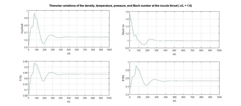
Figure 5: Timewise variations of the density, temperature, pressure, and Mach number at the nozzle throat
In time marching the values of variables changes from previous time step to next time step and these changes tends to becomes smaller and smaller as solution march in time. When flow variables no longer show any significant change in values then it is said to be achieved a steady state. The patterns these variables at the throat taken during a time marching is shown in figure 5 .
The figure 5, shows a large oscillations in the values at initial time steps and the values are settling down in later time steps slowly and after approximately 600 iterations the changes in variables are very small. In early time period the predicted values of variables are far from the actual values so this difference is marked by large variation on plot. The value of property at t+`Delta`t is given by
`rho overset(t+Deltat)``= rho oversett``+ ((delrho)/(delt))overset(t)(avg)`
and
`((delrho)/(delt))overset(t)(avg) = rho overset(t+Deltat)- rho oversett`
here `((delrho)/(delt))overset(t)(avg)` is the difference in actual and predicted value and which is called the residual . As the value of residual goes down solution reach near to the actual value. The value of derivative at start are very high due some unsteady compression and expansion waves which are propagating in nozzle during transient process. The value these derivatives grows smaller and smaller in later time steps.
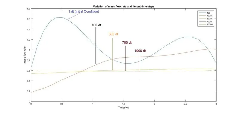
Figure 6: Instantaneous distributions of the non-dimensional mass flow as a function of distance through nozzle at five
different instances during time marching.
Figure 6, shows non-dimensional mass flow is plotted aginst non dimensional distance at different instances of time i.e iterations. This plot explains how with timewise variation of flow properties steady state is achieved for mass flow variation.
- Line cooresponding to 1dt i.e first itearation shows the masss flow variation partaining to initially assumed values of density, velocity and and area ratio. As solution marches forward in time the mass flow rate variation kind of begin to settle down at 100 dt , as solution recheas to 700 dt the mass flow is almost a flat with very small variation which chan be neglected and it is said that mass flow is converged to a constant steady value.
2. Conservative form:
The conservative form of governing equation is solved by converting it into a generic form. The variation of primitve variables obtained from generic variables agianst non-dimensional distance is plotted in figure 7. These variable shows similar behaviors as that obtained by solving conservative form of governing equation.
Figure 7:Variation of primitive variables
Variation of non-dimensional mass flow rate is as shown in figure 8. The variation in values is very small ( considering values upto three decimal points ) due to numerical round off during the formulation.
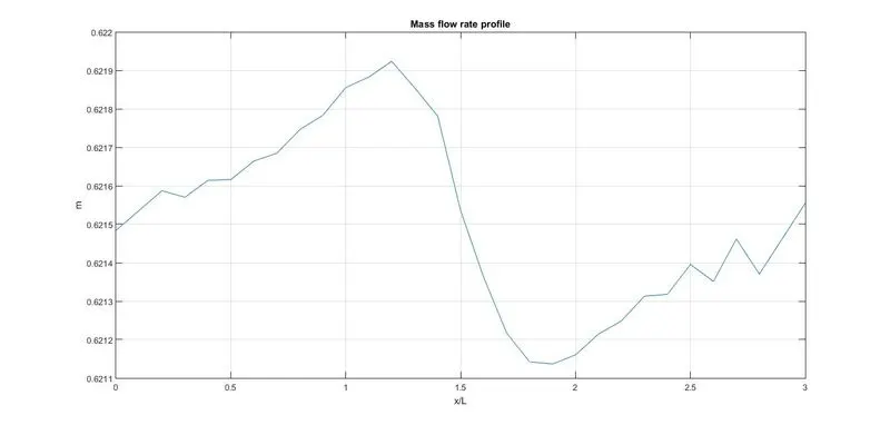
Figure 8: Mass flow rate profile across the one-dimensional Nozzle length
Time wise variation of primitive variables at node number 16 i. throat is shown in figure 9, Property variables undergo large variation during early development of solution follwed by gradual decrease in fluctuation and values settling down to almost constant values in later time. Steady state values achieved by these variables are almost same as that of achieved by solving non conservative form.
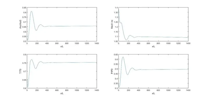
Figure 9: Timewise variations of the density, temperature, pressure, and Mach number at the nozzle throat
3. Conclusions:
1. Figure 10, shows comparison for steady mass flow rate distribution predicted by non-conservative and conservative form.
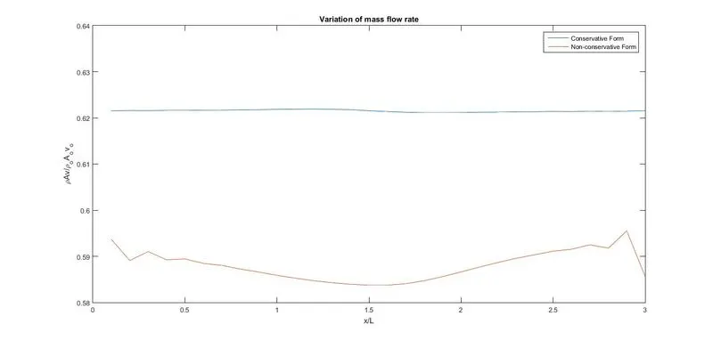
Figure 10: Comparison of the steady-state mass flow variations (on a magnified scale) obtained with the
nonconservat10n and conservation forms of the governing flow equations
Mass flow rate distribution predicted by conservation form is much close of being contant as compared to non conservative form in which some fluctuation are observed at inlet and exit.
- Conservative form does good because mass flow itself is dependent variable (U2) in conservative formulation therefore, mass flow is primary result unlike in non-conservative form where mass flow is obatined as secondary result.But practically both can be considered to be giving constant mass flow rate distribution.
2. When same initial conditions are used for both forms it is observed that ovrall the non conservative form gives a steady state mass flow rate much closer to exact analytical solution i.e m= 0.579
3. Non conservation form does good in terms of residuals as compared to conservative form.
|
Residual |
drhodt_avg |
dU2_dt_avg |
|
Iterations |
Non-conservative Form |
Conservative Form |
|
1 |
0.1419 |
-0.2 |
|
200 |
-0.0953 |
0.0794 |
|
400 |
0.096 |
0.0058 |
|
600 |
0.0096 |
-0.0001 |
|
800 |
1.1253e-4 |
-3.64e-5 |
|
1000 |
-3.936e-7 |
1.14e-5 |
In early iteration residual for a non-conservative form is of order `10^-1` and as time marches the residual decays to a order of `10^-7` But this decay in case of conservative form is of order of `10^-5` for 1000 iterations. The algorithm which offers smallest value of residuals and faster rate of decay is favorable to use depending on application.
4. Formulating a conservative form takes a bit extra effort for generalistion into generic form and primitv variables are need to be decode from flux variables unlike for non-conservative form.
5. Grid Independence test:
The solution is said to be grid-independent when number of grid points are changed the values of variable are same or difference in values is within acceplatble limit.In this example grid independence test is performed by increasing number of grid points from 31 to 61 and effect is seen at the location of minimum areai.e throat. Doubling the grid point did improve values of variables but marginally. this is true for all loctions inside nozzle. These values are not same as that analytical solution but more close to it as shown in table below;
Non-conservative form:
| n =61 | ||||
|
A/Ao |
`rho/(rhoo)` | T/To | P/Po | M |
|
1 |
0.6398 | 0.8365 | 0.5352 | 0.9996 |
|
n= 31 |
||||
| 1 | 0.6386 | 0.8364 | 0.5342 | 0.9994 |
Conservative form
| 1 | 0.6579 | 0.7531 | 0.4955 | 1.0885 |
Analytical Solution
| 1 | 0.6339 | 0.8333 | 0.5282 | 1 |
The variation in value is approximately 1% which is within the accepatble limit for this problem . So this solution corresponding to 31 grid point is grid-independent. This acceptable limit may vary depending on nature of problem and accuracy required.
6. In terms of accuracy both forms yeilds satisfactory results (close to analytical solution) , non conservative form produces slightly accuarte results in terms of primitive variables and conservative form gives slightly more accuarte result for flux values.
7. In this problem pressure at exit is function of pressure at internal node adjacent to exit, pressure is output of boundary condition and flow field inside of nozzle. But if prssure at exit (Pe) is specified and Pe is maintained such that (Pe/P0) > 0.0163 then, the presence of shock will be there in diverging section (supersonic flows are prone to shocks) which will affect the values of all primitive variables. In that case shock capturing will be critical.