Week 8 - Simulating Cyclone separator with Discrete Phase Modelling
Simulating Cyclone Separator with Discrete Phase Modelling
Aim:
To Perform the analysis on the Cyclone separator and calculate the separation efficiency and pressure drop with varying the particle diameter and particle velocity.
Objective:
- To write a few words about any four empirical models used to calculate the cyclone separator efficiency.
- To perform an analysis on a given cyclone separator model by varying the particle diameter from 1 µm to 5µm and calculate the separation efficiency in each case. Discuss the results. [Use both the velocity's as 3 m/sec.]
- To perform an analysis on a given cyclone separator model by varying the particle velocity from 1 m/sec to 5 m/sec and calculate the separation efficiency and pressure drop in each case. Discuss the results. [Use particle diameter size as 5 µm for all cases & keep flow velocity same as particle velocity]
Boundary conditions:
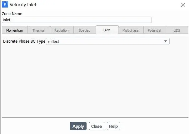
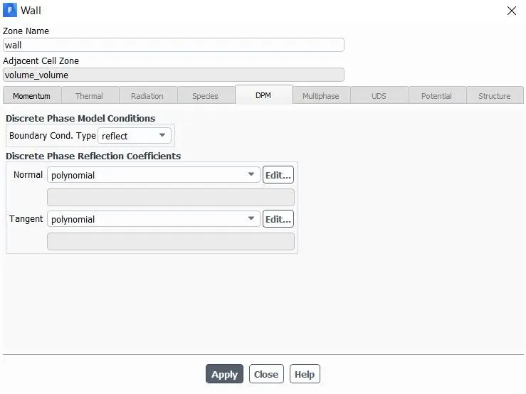
Inlet and wall = Reflect
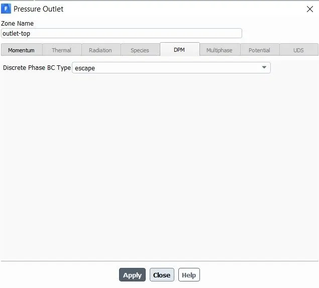
Outlet (Top) = Escape
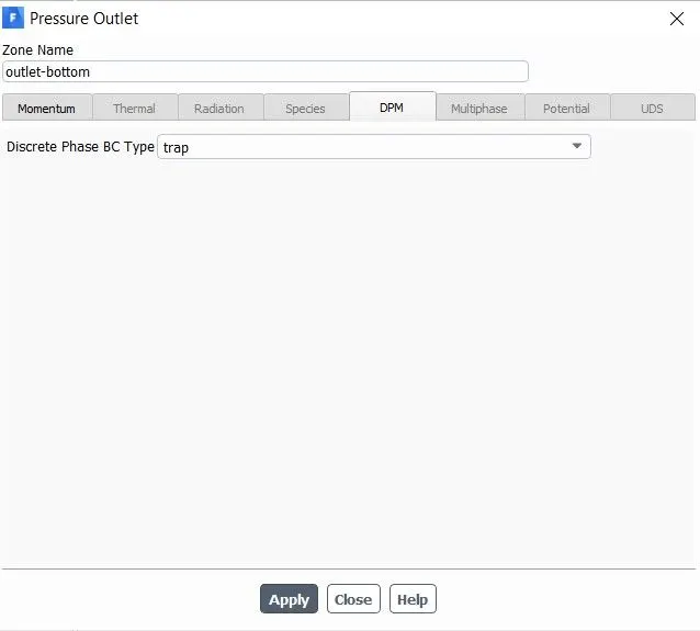
Outlet (Bottom) = Trap
Introduction And Theory:-
Cyclone Separator:-
Cyclone Separation is a method of removing particulates from an air, gas or liquid stream, without the use of filters, through vortex separation. When removing particulate matter from liquid, a hydro cyclonic is used; while from gas, a gas cyclone is used. Rotational effects and gravity are used to separate a mixture of solids and fluids. The method can also be used to separate fine droplets of liquid from the gaseous stream.
Discrete Phase Modelling:-
A discrete phase model (DPM) is used when the aim is to investigate the behaviour of the particles from the Lagrangian view and a discrete perspective. In fact, the difference between the Lagrangian and the Eulerian view is that fluid behaviour in the Lagrangian view is examined on the basis of a particle tracking of a particle of fluid flow Whereas fluid behaviour is considered in the Eulerian view based on the assumption of a finite volume element in the fluid flow path.
If the behaviour of discrete particles in the presence of a continuous flow field is affected by continuous flow, the interaction with the continuous phase must be activated. The discrete phase can be applied in various physical forms, the type of which depends on the problem model. One of the physical defining models is the two-way turbulent coupling mode, which is used to study the effects of change in the turbulent quantities caused by particle damping and Eddy turbulence.
Injection:-
The Injection process for the mixed flow is defined in the input section of the model. In this way, in the input section of the model, the desired material enters the interior space of the model with the same discrete state or particle by particle. The particle injection as a discrete state can occur in different states. For example, the combustion mode is used when the material is injected into the model's interior to perform the combustion process.
Empirical Models of Cyclone Efficiency:-
- Iozia and Leith Model
- Li and Wang Model
- Koch and Licht Model
- Lapple Model
Iozia and Leith Model:-
Iozia and Leith logistic model is a modified version of Barth Model, Which is developed based on force balance. The model assumes that a particle carried by the vortex endures the influence of two forces: a centrifugal force, Z and a flow resistance, W. The collection efficiency `eta_i` of paricle diameter `d_"pi"` can be calculated from
`eta_i = (1)/(1+(d_(pc)//d_"pi")^beta)`
`beta` is an expression for slope parameters derived based on the statistical analysis of experimental data of a cyclone with D = 0.25 m given as
`beta = 0.62-0.87ln (d_(pc)/100) + 5.21ln ((ab)/(D^2)) + 1.05[ln((ab)/(D^2))]^2`
and `d_(pc)` is the 50% cut size given by barth
`d_(pc) = [(9muQ)/(pi rho_p Z_c V_(i max )^2)]^0.5`
Where core length `Z_c` ,and core diameter, `d_c` are given as
`Z_c = (H - S) [(H-S)/((D//B) - 1)] [(d_c//B)-1]` for `d_c >B`
`Z_c = H-S` for `d_c< B`
`d_c = 0.47D((ab)/D^2)^-0.25 (D_e/D)^1.4`
Li and Wang Model:-
The Li and Wang model include particle bounce or re-entrainment and turbulent diffusion at the cyclone wall. A two-dimensional analytical expression of particle distribution in the cyclone is obtained. Li and Wang model was developed based on the following assumptions.
- The radial particle velocity and the radial concentration profile are not constant for uncollected particles within the cyclone.
- Boundary conditions with the consideration of turbulent diffusion coefficient and particle bounce re-entertainment on the cyclone wall.
- The Tangential velocity is related to the radius of cyclone by: u`R^n` = constant
Koch and Licht Model:-
Koch and Licht collection theory recognized the inherently turbulent nature of cyclones and the distribution of gas residence times within the cyclone. Koch and Licht described particle motion in the entry and collection regions with the additional following assumptions:
- The tangential velocity of a particle is equal to the tangential velocity of the gas flow. i.e there is no slip in the tangential direction between the particle and the gas.
- The tangential velocity is related to the radius of cyclone by: u `R^n` = constant
Lapple Model:-
Lapple model was developed based on force balanced without considering the flow resistance. Lapple assumed that a particle entering the cyclone is evenly distributed across the inlet opening. The particle that travels from the inlet half-width to the wall in the cyclone is collected with 50% efficiency. The semiempirical relationship developed by Lapple to calculate a 50% cut diameter. `d_(pc)`,is
`d_(pc) = [ (9mu b)/(2piN_e v_i(rho_p - rho_g))]^(1/2)`
where `N_e` is the number of revolutions
`N_e = 1/a[h+(H-h)/2]`
The efficiency of collection of any size of particle is given by
`eta_i = 1/ (1+(d_(pc)//bar d_"pi")^2`
Simulation Process:-
The analysis of a given model is to varying the diameter of particle size and varying the particle velocity.
Part-1:- Varying the Diameter of particle size.
- Case - 1 => Particle Diameter 1 µm
- Case - 2 => Particle Diameter 2 µm
- Case - 3 => Particle Diameter 3 µm
- Case - 4 => Particle Diameter 4 µm
- Case - 5 => Particle Diameter 5 µm
Part-2:- Varying the Particle Velocity.
- Case - 6 => Velocity 1 m/s
- Case - 7 => Velocity 2 m/s
- Case - 8 => Velocity 3 m/s
- Case - 9 => Velocity 4 m/s
- Case - 10 => Velocity 5 m/s
Geometry:-
- In SpaceClaim the given geometry(cyclone separator) is loaded.
- And the Fluid volume is extracted.
- The cyclone separator has been disabled and Suppress for physics for further simulation.
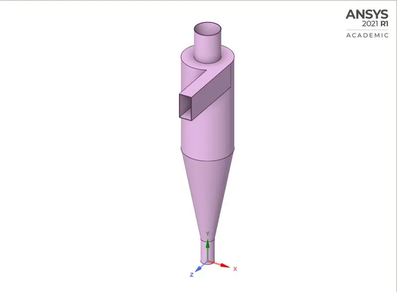
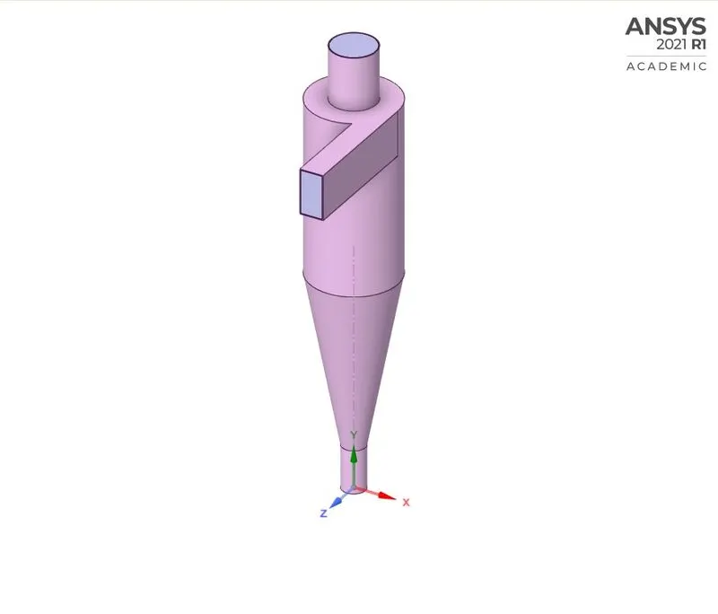
Fig(a). Cyclone Separator Fig(b). Fluid Volume and cyclone separator
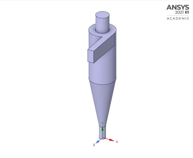
Fig(c). Fluid volume extracted geometry
Meshing:-
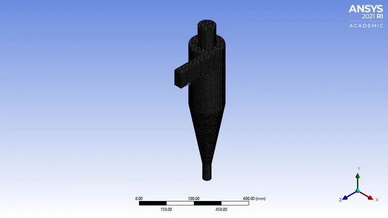
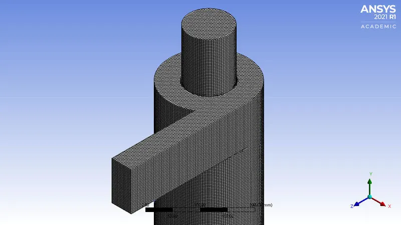
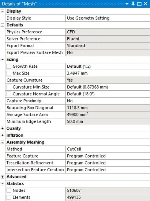
- In Meshing the Cutcell meshing approach is used for the structural mesh which gives better results.
- The Cutcell mesh is available in Assembly meshing.
- The named selection is given as Inlet, Outlet (Top), Outlet (Bottom), Wall.
Meshing Details
- Method = Cutcell
- Max Size = 3.4947 mm
- Nodes = 510607
- Elements = 499135
Named Selection:-
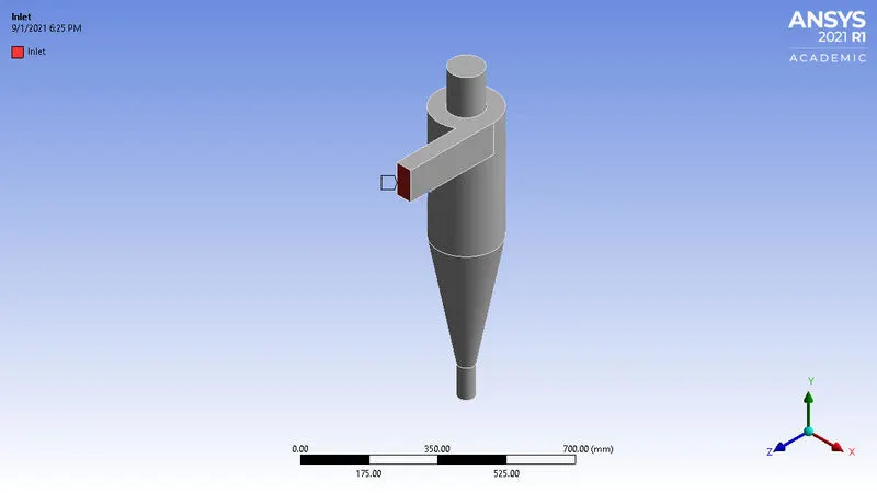
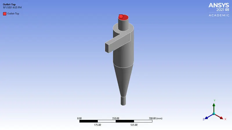
Fig(a). Inlet Fig(b). Outlet (Top)
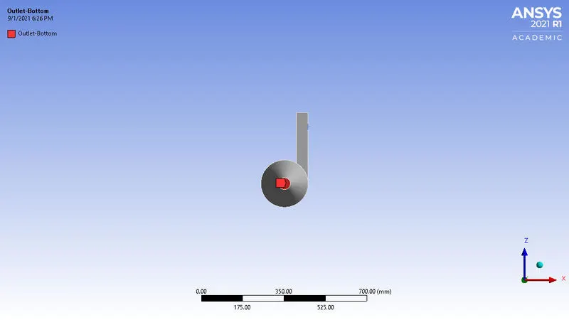
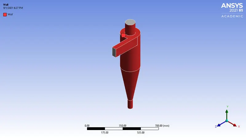
Fig(c). Oulet (Bottom) Fig(d). Walls
Fluent Setup:-
1. Type = Presure Based Solver
2. Velocity Formulation = Absolute.
3. Time = Steady state
4. Gravity = -9.81 in y-direction
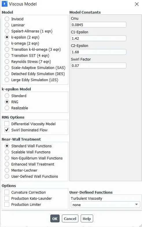
5. Viscous model = K-Epsilon, RNG Model, Swirl Dominated Flow
6. Discrete Phase Model.
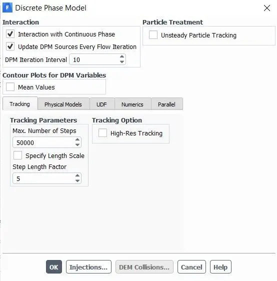
7. Boundary Condition For DPM (Discrete phase model)
a. Inlet and Walls = Reflects
b. Outlet (Top) = Escape
c. Outlet (Bottom) = Trap
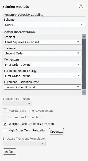
8. Solution Methods:-
9. Initialization.
- Standard initialization compute from Inlet
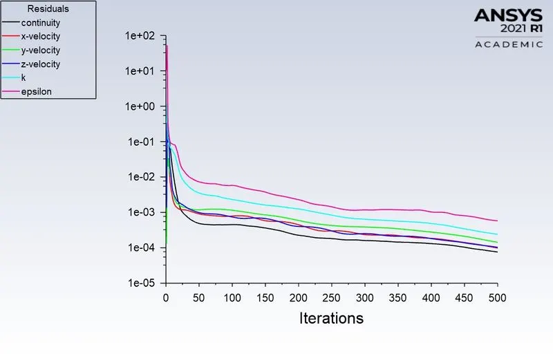
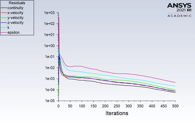
- Run for 500 iterations.
\*******************************************************************************************************************************************************/
Part-1:- Varying the Diameter of particle size.
Case-1:- Particle Diameter 1 µm
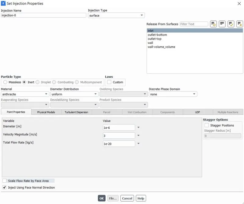
Injection Properties:-
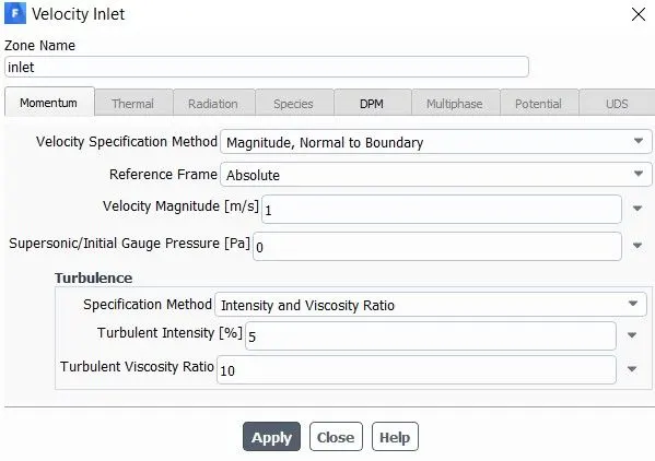
Boundary condition (Inlet Velocity):-
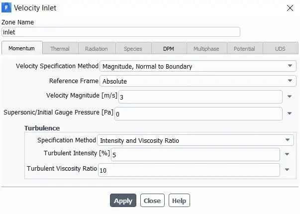
The velocity is used 3 m/s for case-1 to case-5.
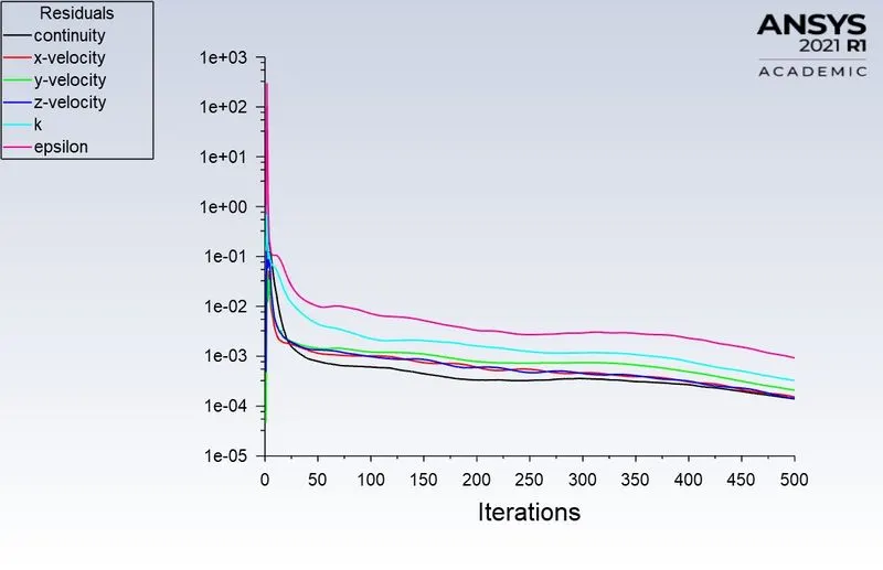
Scaled Residuals:-
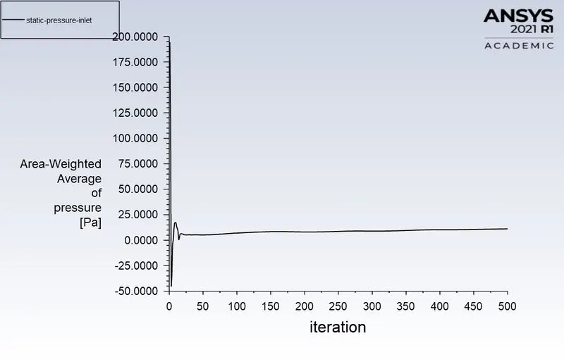
Static Pressure (Inlet):-
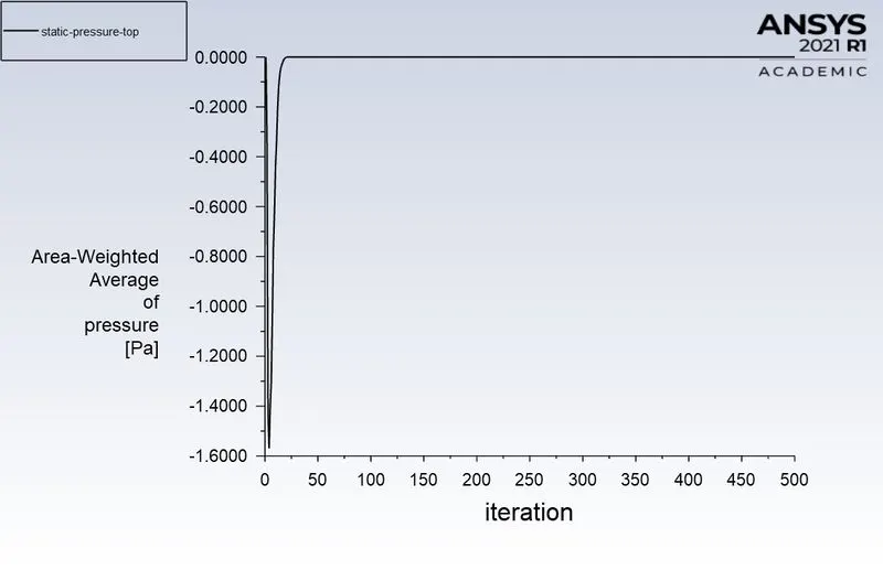
Static Pressure (Top):-
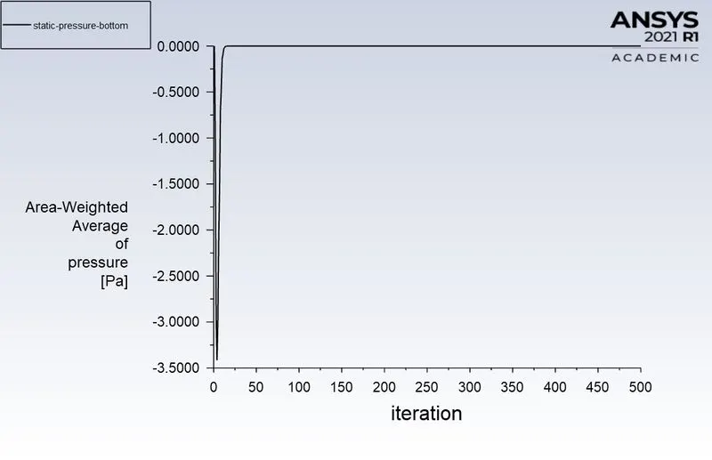
Static Pressure (Bottom):-
Separation Efficiency:-

`"Separation efficiency" = "No. of Particles Trapped"/"No. of Particles Tracked"`
`"Separation Efficiency" = 209/435`
`"Separation Efficiency" = 48.04%`
Pressure Drop:-
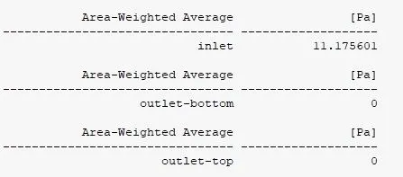
`"Pressure Drop" = ("Inlet Pressure of the Fluid - Outlet Pressure of the Fluid")`
`"Pressure Drop" = (11.17 - 0)`
`"Pressure Drop = 11.17 Pa"`
∴ The Inlet Pressure is equal to pressure drop. Because the Outlet pressure is maintained as 0 Pascal. And the Pressure Drop for Case 1-5 is same as 11.17 Pa because the velocity cannot change. The velocity is directly proportional to pressure.
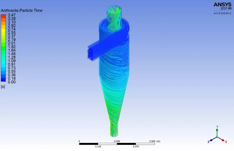
Anthracite Particle Time:-
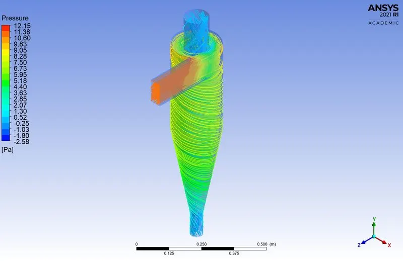
Pressure:-
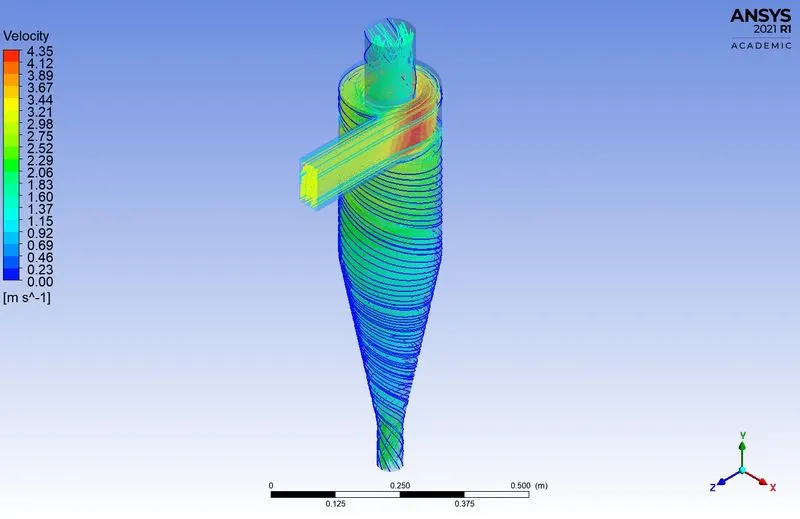
Velocity:-
\*******************************************************************************************************************************************************/
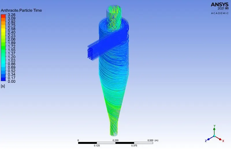
Case - 2 => Particle Diameter 2 µm
Injection Properties:-
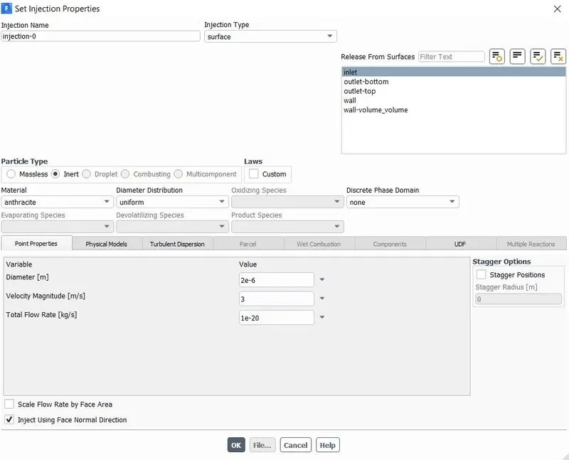
Scaled Residuals:-
Separation Efficiency:-

`"Separation efficiency" = "No. of Particles Trapped"/"No. of Particles Tracked"`
`"Separation Efficiency" = 225/435`
`"Separation Efficiency" = 51.72%`
Anthracite Particle Time:-
\*******************************************************************************************************************************************************/
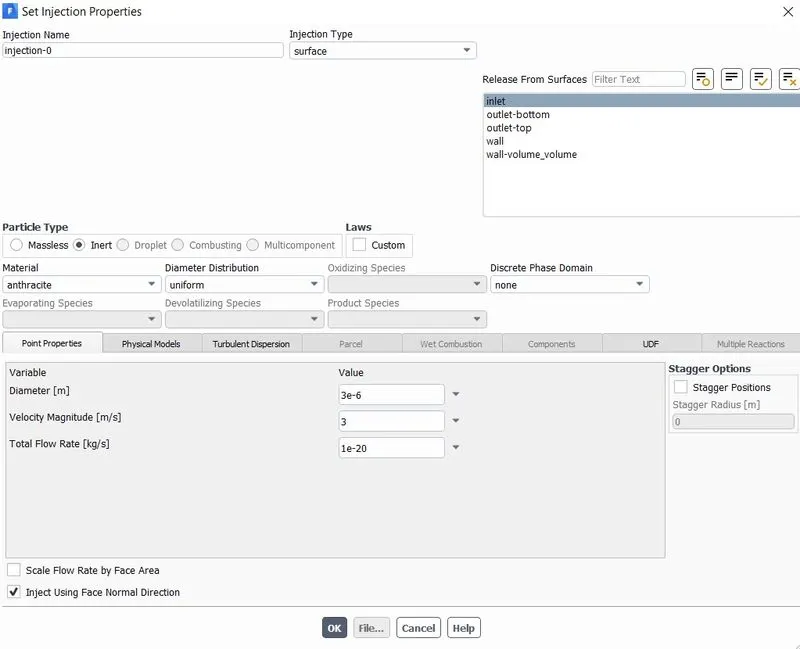
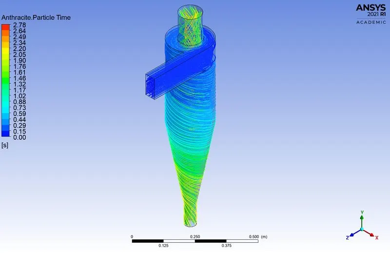
Case - 3 => Particle Diameter 3 µm
Injection Properties:-
Scaled Residuals:-
Separation Efficiency:-

`"Separation efficiency" = "No. of Particles Trapped"/"No. of Particles Tracked"`
`"Separation Efficiency" = 241/435`
`"Separation Efficiency" = 55.40%`
Anthracite Particle Time:-
\*******************************************************************************************************************************************************/
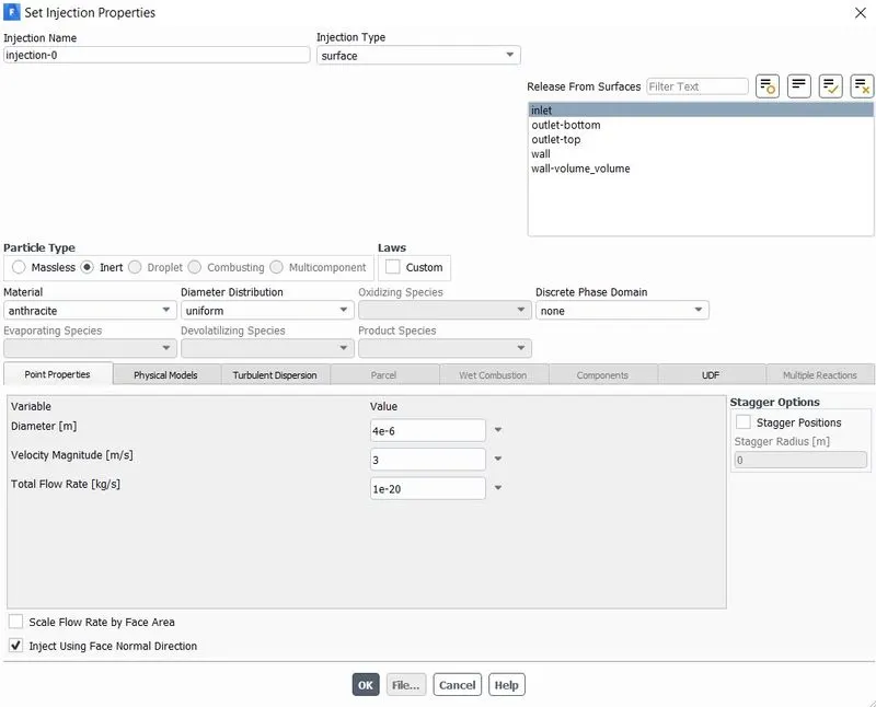
Case - 4 => Particle Diameter 4 µm
Injection Properties:-
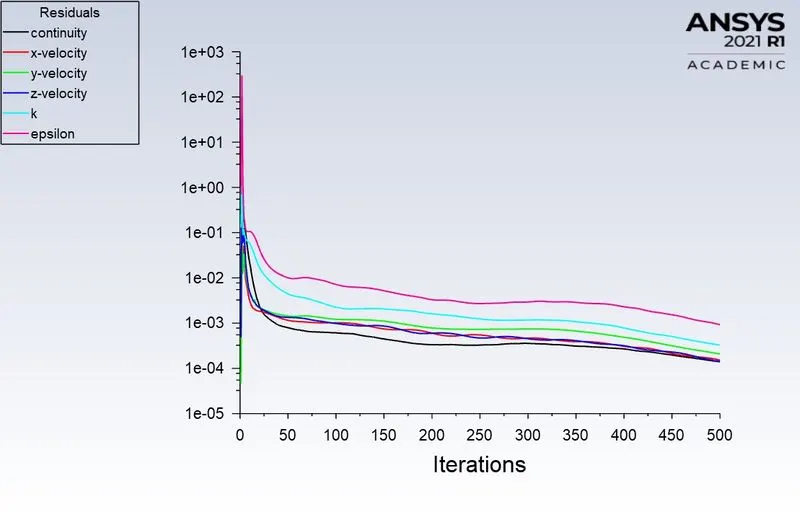
Scaled Residuals:-
Separation Efficiency:-

`"Separation efficiency" = "No. of Particles Trapped"/"No. of Particles Tracked"`
`"Separation Efficiency" = 273/435`
`"Separation Efficiency" = 62.75%`
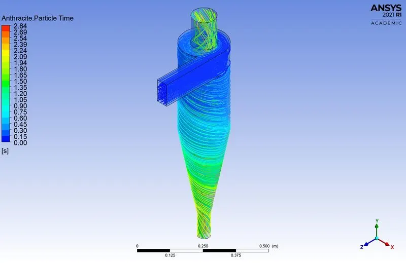
Anthracite Particle Time:-
\*******************************************************************************************************************************************************/
Case - 5 => Particle Diameter 5 µm
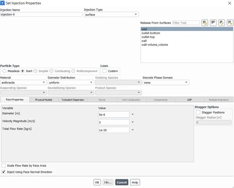
Injection Properties:-
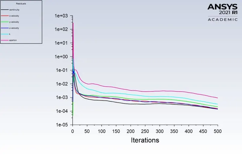
Scaled Residuals:-
Separation Efficiency:-

`"Separation efficiency" = "No. of Particles Trapped"/"No. of Particles Tracked"`
`"Separation Efficiency" = 309/435`
`"Separation Efficiency" = 71.03%`
Anthracite Particle Time:-
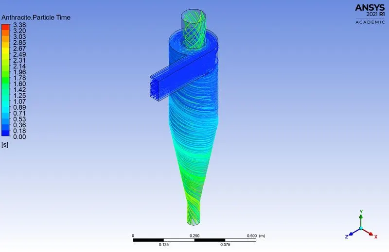
Animation:-
\*******************************************************************************************************************************************************/
Part-2:- Varying the Particle Velocity
Case - 6 => Velocity 1 m/s
Injection Properties:-
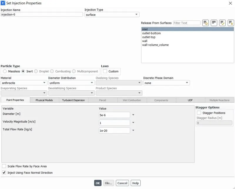
Boundary condition (Inlet Velocity):-
Scaled Residuals:-
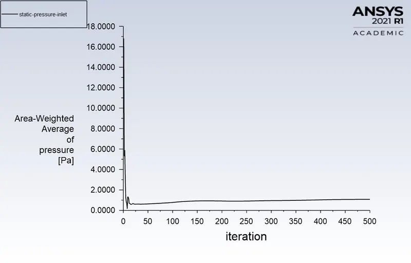
Static Pressure (Inlet):-
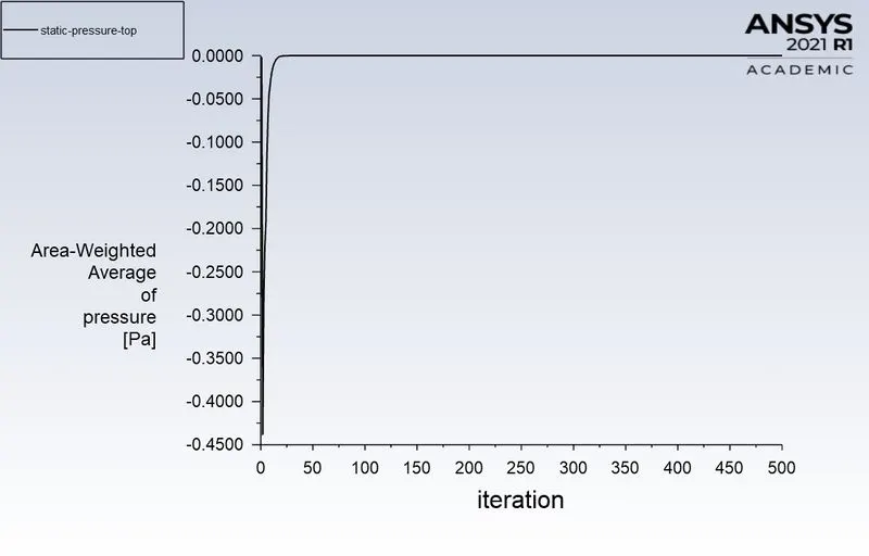
Static Pressure (Top):-
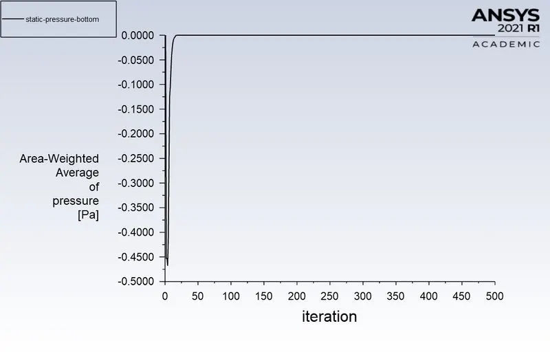
Static Pressure (Bottom):-
Separation Efficiency:-

`"Separation efficiency" = "No. of Particles Trapped"/"No. of Particles Tracked"`
`"Separation Efficiency" = 118/435`
`"Separation Efficiency" = 27.12%`
Pressure Drop:-
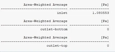
`"Pressure Drop" = ("Inlet Pressure of the Fluid - Outlet Pressure of the Fluid")`
`"Pressure Drop" = (1.08 - 0)`
`"Pressure Drop = 1.08 Pa"`
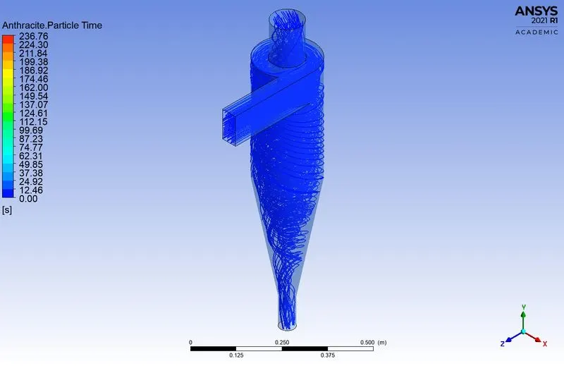
Anthracite Particle Time:-
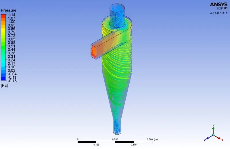
Pressure:-
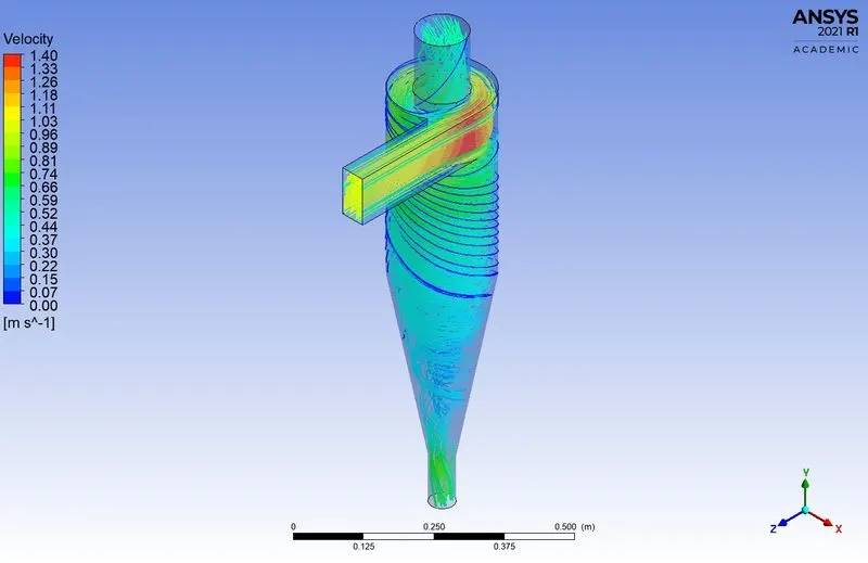
Velocity:-
\*******************************************************************************************************************************************************/
Case - 7 => Velocity 2 m/s
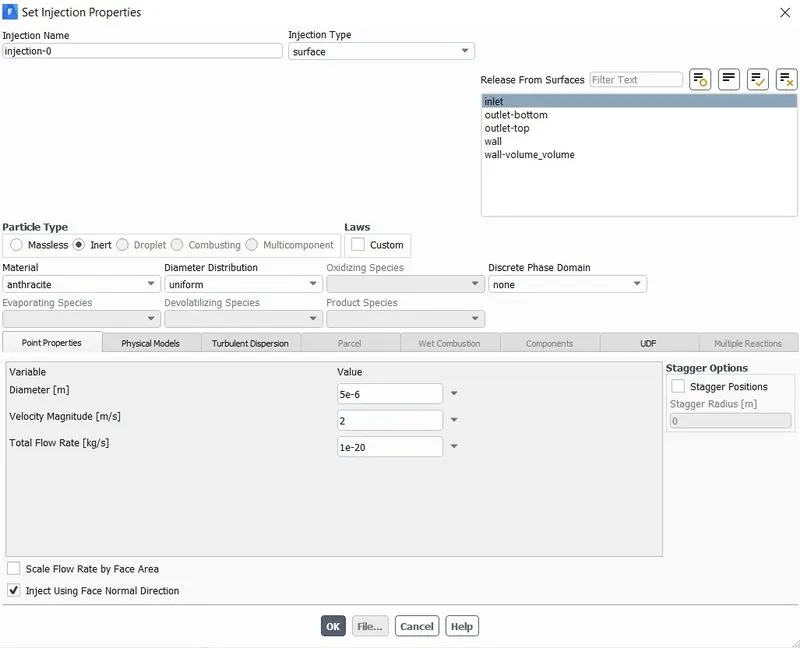
Injection Properties:-
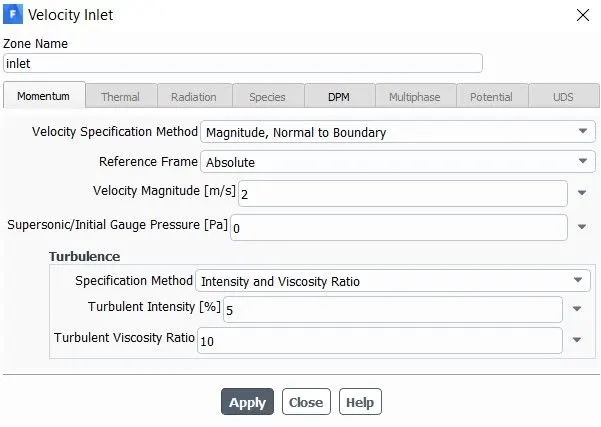
Boundary condition (Inlet Velocity):-
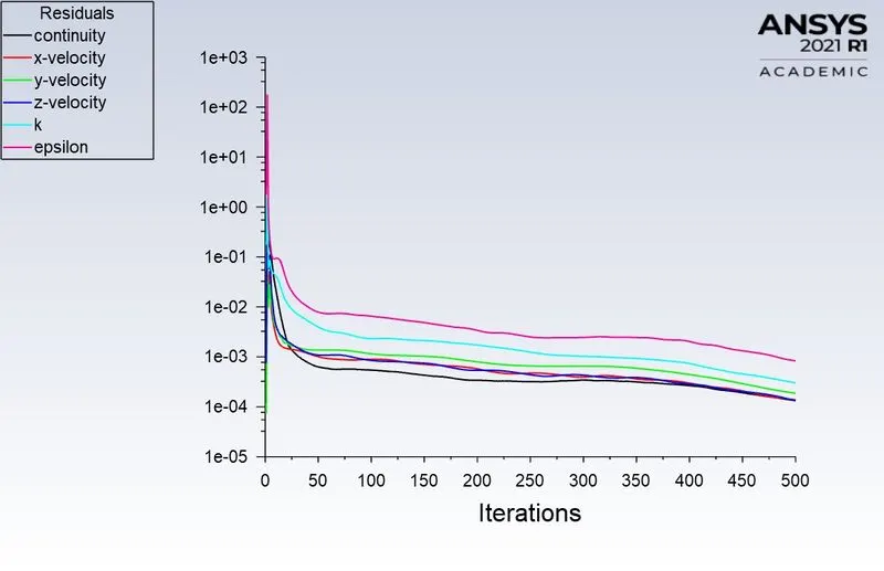
Scaled Residuals:-
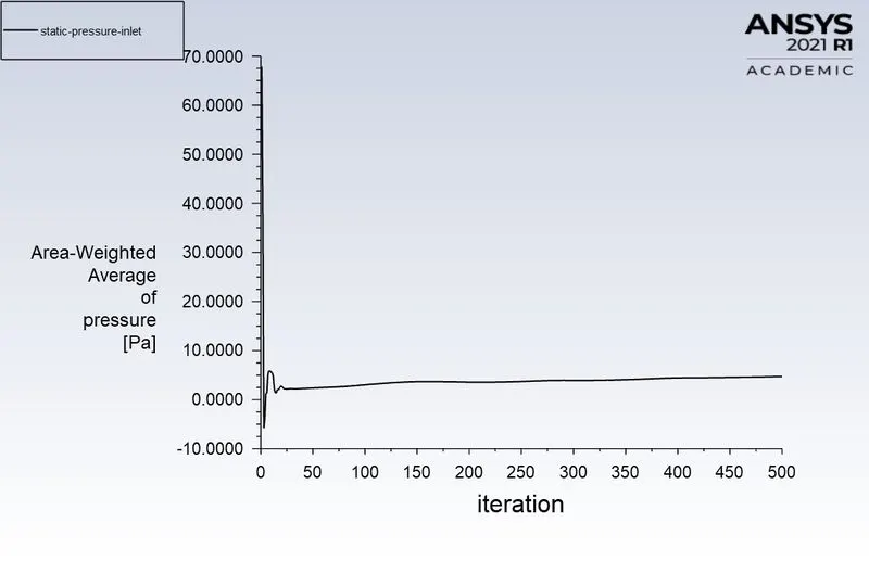
Static Pressure (Inlet):-
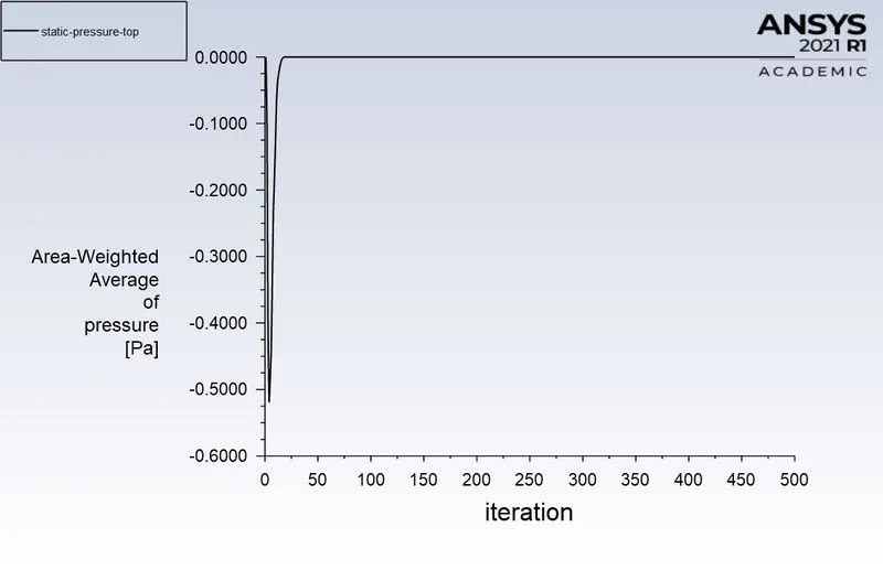
Static Pressure (Top):-
Static Pressure (Bottom):-
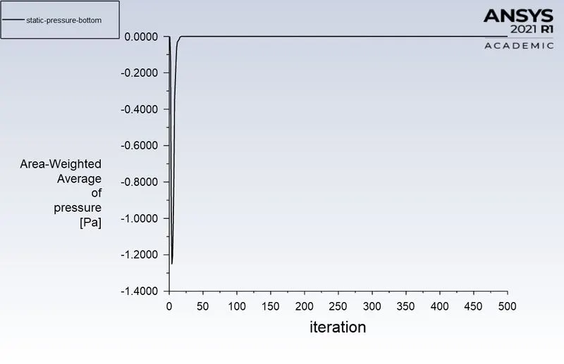
Separation Efficiency:-

`"Separation efficiency" = "No. of Particles Trapped"/"No. of Particles Tracked"`
`"Separation Efficiency" = 265/435`
`"Separation Efficiency" = 60.92%`
Pressure Drop:-
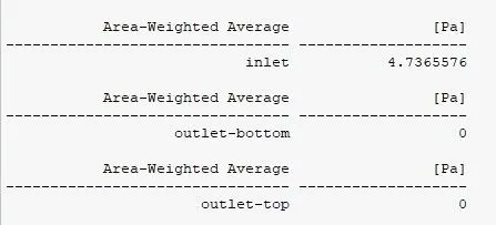
`"Pressure Drop" = ("Inlet Pressure of the Fluid - Outlet Pressure of the Fluid")`
`"Pressure Drop" = (4.73 - 0)`
`"Pressure Drop = 4.73 Pa"`
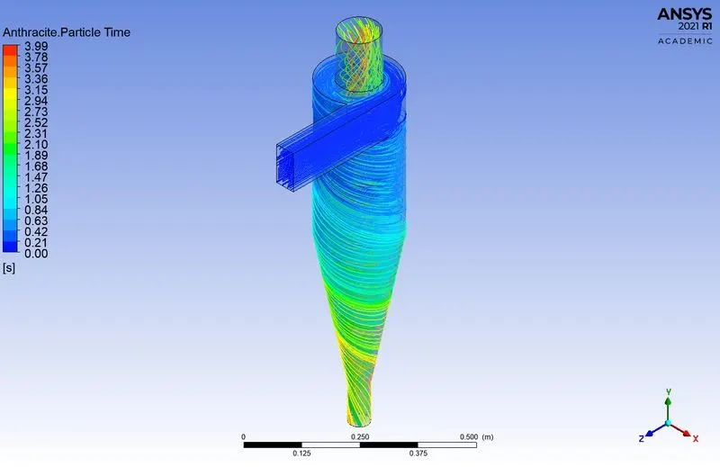
Anthracite Particle Time:-
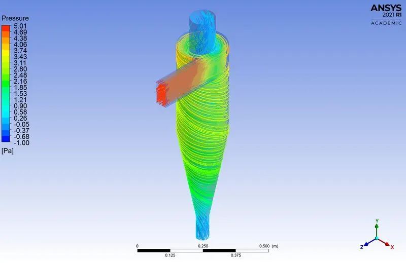
Pressure:-
Velocity:-
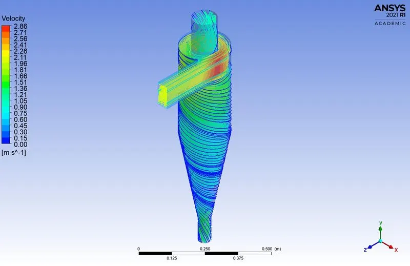
\*******************************************************************************************************************************************************/
Case - 8 => Velocity 3 m/s
Injection Properties:-
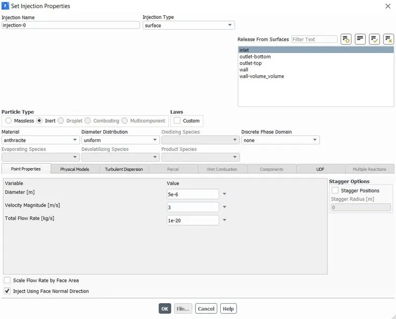
Boundary condition (Inlet Velocity):-
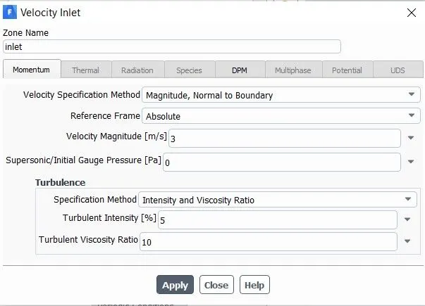
Scaled Residuals:-
Static Pressure (Inlet):-
Static Pressure (Top):-
Static Pressure (Bottom):-
Separation Efficiency:-

`"Separation efficiency" = "No. of Particles Trapped"/"No. of Particles Tracked"`
`"Separation Efficiency" = 309/435`
`"Separation Efficiency" = 71.03%`
Pressure Drop:-
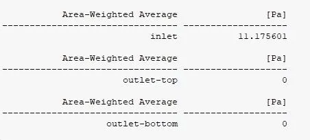
`"Pressure Drop" = ("Inlet Pressure of the Fluid - Outlet Pressure of the Fluid")`
`"Pressure Drop" = (11.17 - 0)`
`"Pressure Drop = 11.17 Pa"`
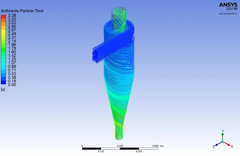
Anthracite Particle Time:-
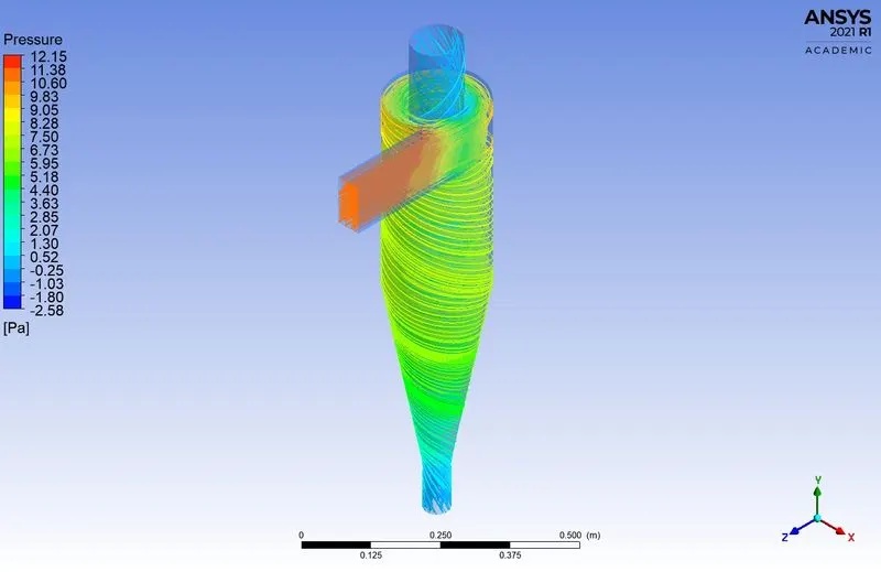
Pressure:-
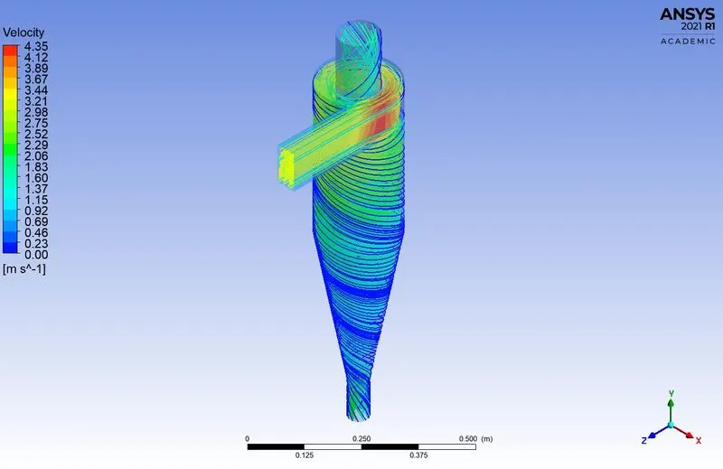
Velocity:-
\*******************************************************************************************************************************************************/
Case - 9 => Velocity 4 m/s
Injection Properties:-
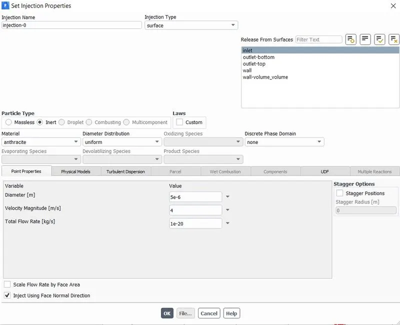
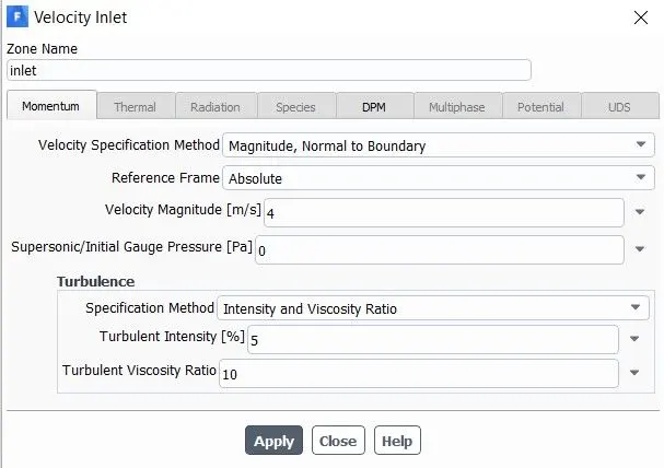
Boundary condition (Inlet Velocity):-
Scaled Residuals:-
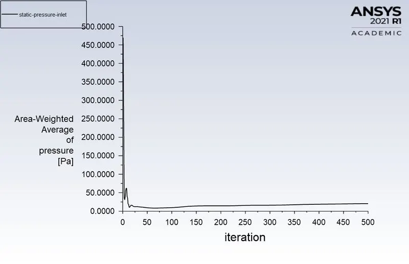
Static Pressure (Inlet):-
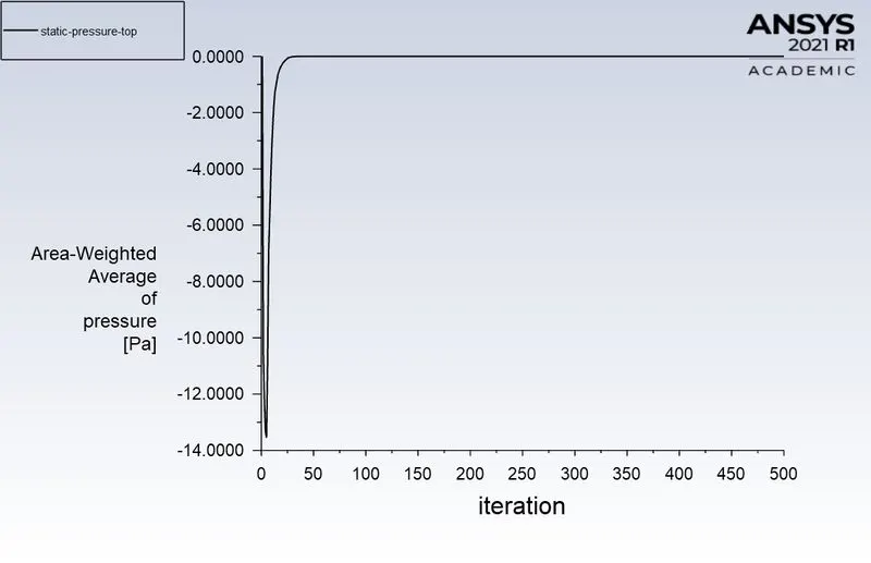
Static Pressure (Top):-
Static Pressure (Bottom):-
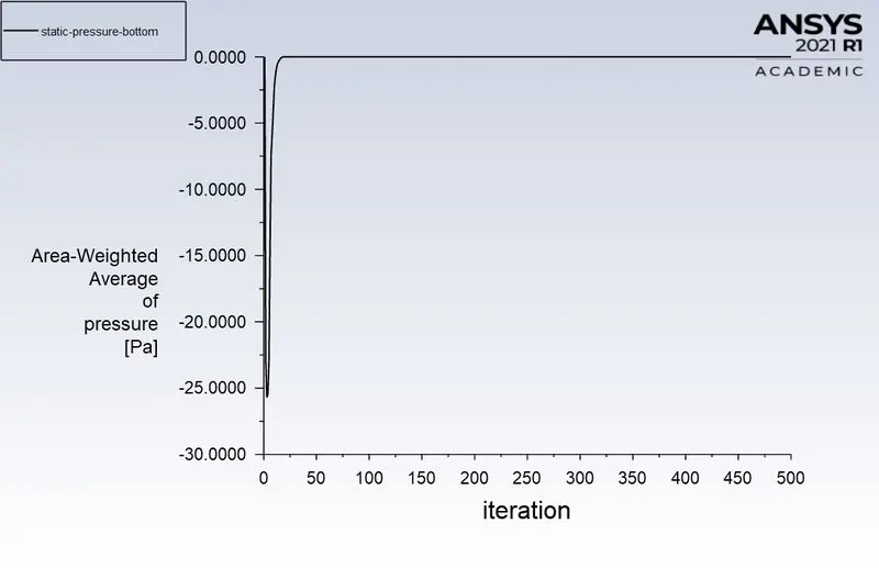
Separation Efficiency:-

`"Separation efficiency" = "No. of Particles Trapped"/"No. of Particles Tracked"`
`"Separation Efficiency" = 341/435`
`"Separation Efficiency" = 78.39%`
Pressure Drop:-
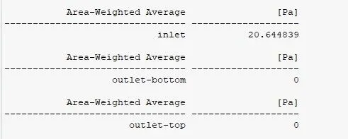
`"Pressure Drop" = ("Inlet Pressure of the Fluid - Outlet Pressure of the Fluid")`
`"Pressure Drop" = (20.64 - 0)`
`"Pressure Drop = 20.64 Pa"`
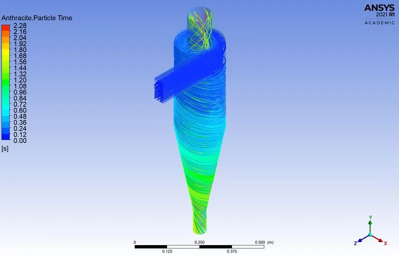
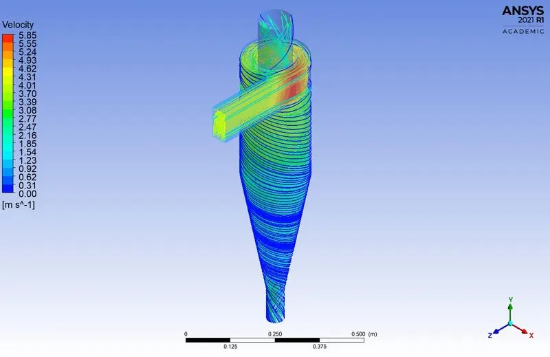
Anthracite Particle Time:-
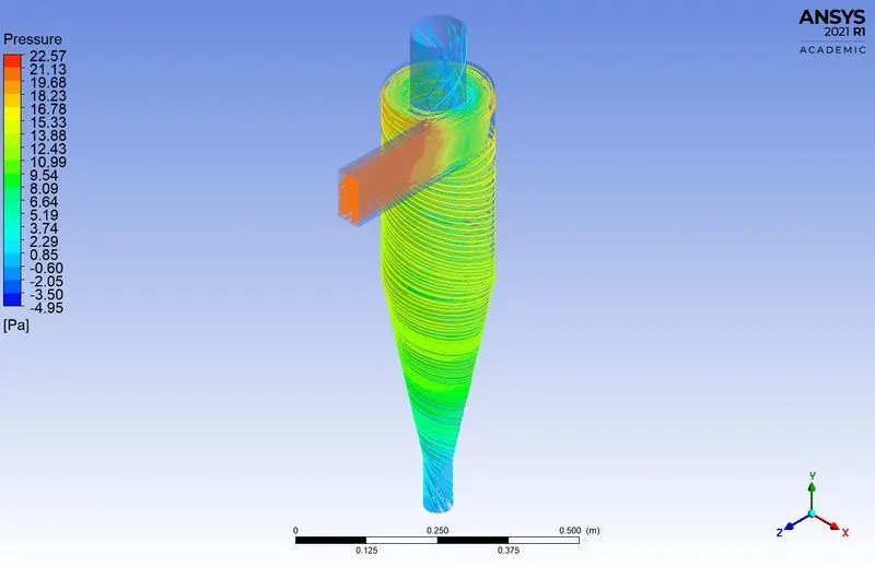
Pressure:-
Velocity:-
\*******************************************************************************************************************************************************/
Case - 10 => Velocity 5 m/s
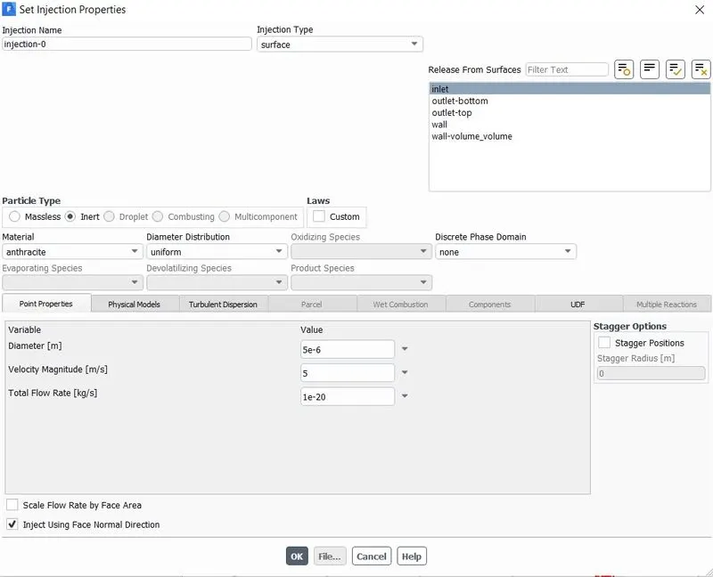
Injection Properties:-
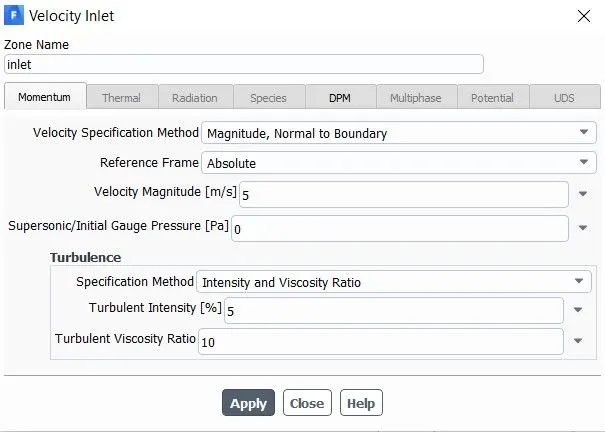
Boundary condition (Inlet Velocity):-
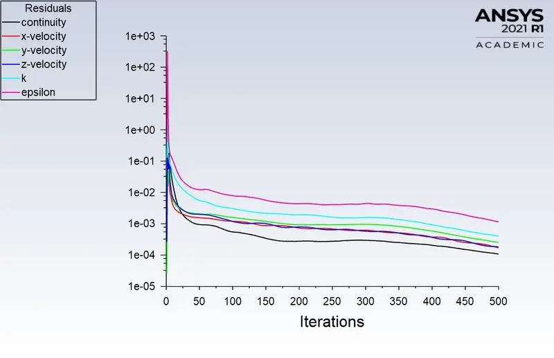
Scaled Residuals:-
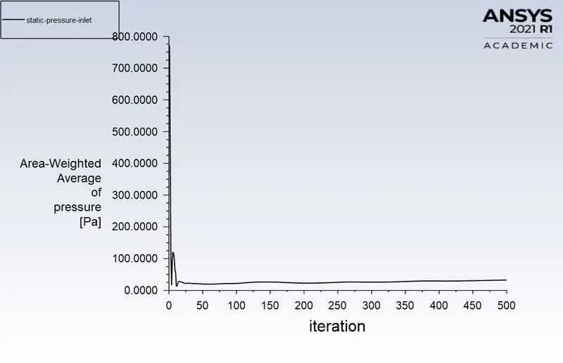
Static Pressure (Inlet):-
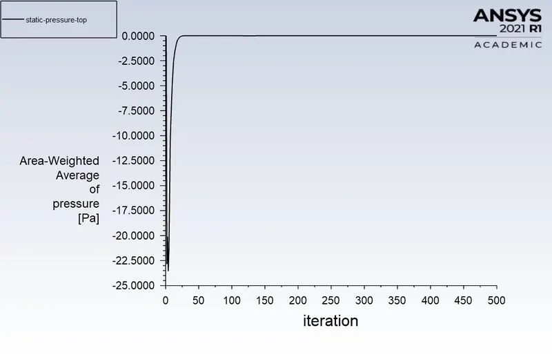
Static Pressure (Top):-
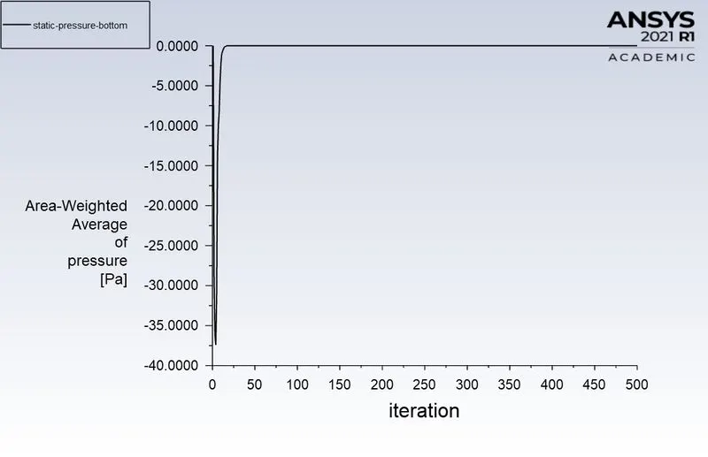
Static Pressure (Bottom):-
Separation Efficiency:-

`"Separation efficiency" = "No. of Particles Trapped"/"No. of Particles Tracked"`
`"Separation Efficiency" = 375/435`
`"Separation Efficiency" = 86.20%`
Pressure Drop:-
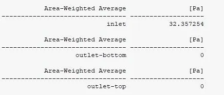
`"Pressure Drop" = ("Inlet Pressure of the Fluid - Outlet Pressure of the Fluid")`
`"Pressure Drop" = (32.35 - 0)`
`"Pressure Drop = 32.35 Pa"`
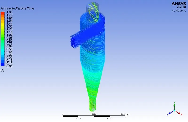
Anthracite Particle Time:-
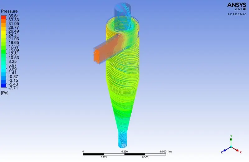
Pressure:-
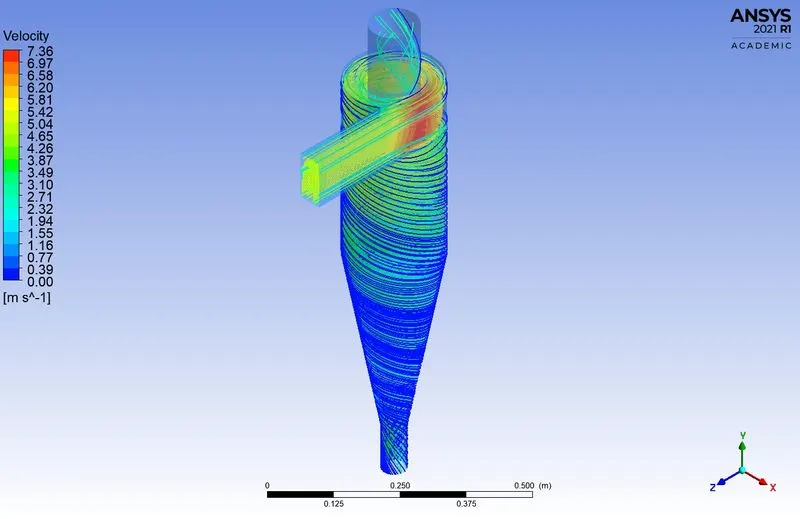
Velocity:-
Animation:-
Vortex core Region:-
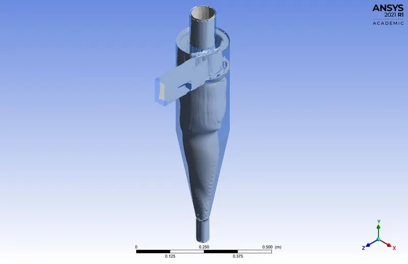
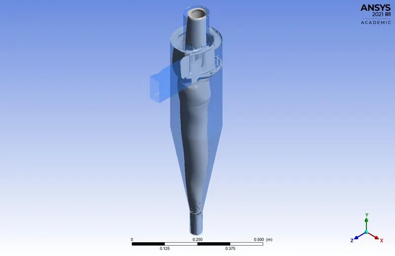
Fig(a). Swirling Strength 0.01 Fig(b). Swirling Strength 0.02
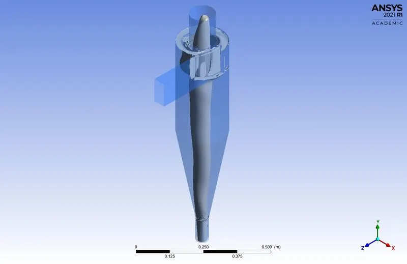
Fig(c). Swirling Strength 0.03
Result and Conclusion:-
Comparison.
| Particle Diameter | Particle Velocity | Particle Tracked | Particle Escaped | Particle Trapped | Particle Incomplete | Separation Efficiency | Pressure Drop | ||
|
Part - 1 (Varying the diameter of particle size) |
Case 1 | 1 µm | 3 m/s | 435 | 214 | 209 | 12 | 48.04 | 11.17 |
| Case 2 | 2 µm | 435 | 210 | 225 | 0 | 51.72 | 11.17 | ||
| Case 3 | 3 µm | 435 | 194 | 241 | 0 | 55.40 | 11.17 | ||
| Case 4 | 4 µm | 435 | 162 | 273 | 0 | 62.75 | 11.17 | ||
| Case 5 | 5 µm | 435 | 126 | 309 | 0 | 71.03 | 11.17 | ||
|
Part - 2 (Varying the Particle velocity) |
Case 6 | 5 µm | 1 m/s | 435 | 217 | 118 | 100 | 27.12 | 1.08 |
| Case 7 | 2 m/s | 435 | 170 | 265 | 0 | 60.92 | 4.73 | ||
| Case 8 | 3 m/s | 435 | 126 | 309 | 0 | 71.03 | 11.17 | ||
| Case 9 | 4 m/s | 435 | 94 | 341 | 0 | 78.39 | 20.64 | ||
| Case 10 | 5 m/s | 435 | 60 | 375 | 0 | 86.20 | 32.35 | ||
- From the above result of the cyclone separator, the efficiency depends upon both the diameter of the particle and the velocity of the particle.
- In part 1 the pressure drop is constant because of no change in velocity. So the pressure drop depends upon the velocity.
- If the particle size is high and velocity is high the efficiency of the cyclone separator is also high.
- At the inlet, the pressure is high because the fluid is injected at high velocity and it will decrease due to swirling.
- And the residence time of particles is reduced when the velocity and diameter are increased.
- If the particle diameter and the velocity is increased the particle escape is reduced and it is collected in the dustbin.