Simulating Cyclone separator with Discrete Phase Modelling

Aim- CFD analysis is conducted on Cyclone separator based on two cases and Ansys fluent is used for setting up the physics of the problem. Results are validated for the separation efficiency obtained for each sub-case.

Cases –

1. To perform an analysis on a given cyclone separator model by varying the particle diameter from 1 μm to 5 μmand calculate the separation efficiency in each case. Discuss the results. [Use both the velocity's as 3m/sec.]
2. To perform an analysis on a given cyclone separator model by varying the particle velocity from 1 m/sec to 5 m/secand calculate the separation efficiency and pressure drop in each case. Discuss the results. [Use particle diameter size as 5 μm for all cases & keep flow velocity same as particle velocity]

Theory –

Cyclone Separator –

Cyclone separators are separation devices (dry scrubbers) that use the principle of inertia to removes particulate matter from the flue gases. Cyclone separator is one of many air pollution removers known as pre-cleaner, since they remove larger piece of particulate matter.

This prevents finer filtration methods from having to deal with large, more abrasive particles later on. In addition several cyclone separator can operator in parallel, and this system is known as a multicyclone.

It is important to note that cyclones can vary drastically in their size. The size of the cyclone depends largely on how much flue gas must be filtered, thus larger operations tend to need larger cyclones. For example, several different models of one cyclone type can exist, and the sizes can range from a relatively small 1.2-1.5 meters tall (about 4-5) to around 9 meters (30-feet) – which is about as tall as a three-story building.

Working –

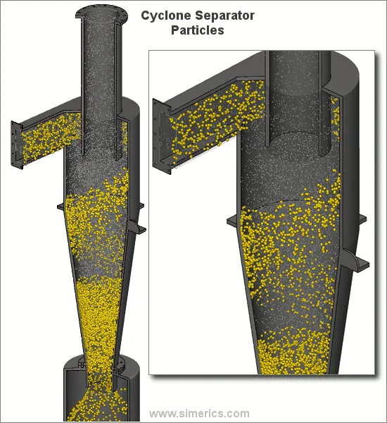
Cyclone separators work much like a centrifuge, but with continuous feed of dirty air. In a cyclone separator, dirty flue gas is fed into a chamber. The inside of the chamber creates a spiral vortex, similar to a tornado. This spiral formation and the separation shown in the figure below. The lighter components of this gas have less inertia, so its easier for them to be influenced by the vortex and travel up it. Contrarily, larger components of particulate matter have more inertia and are not as easily influenced by the vortex.

Since these larger particles have difficulty following the high-speed spiral motion of the gas and the vortex, the particles hit the inside wall of the container and drop down into a collection hopper. These chambers are shaped like an upside-down cone to promote the collection of these particles at the bottom of the container. The cleaned flue gas escapes out the top of the chamber.

Four empirical models used to calculate the cyclone separator efficiency:

IOZIA and LEITH model –

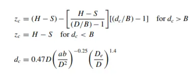
Iozia and leith (1990) model is modified version of Barth (1956) model which is developed based on force balance. The model assumes that a particle carried by the vortex endures the influence of two forces: centrifugal force Z and flow resistance, W. Core length, zc and core diameter are given as:

`n_i=(1)/(1+(dp_c+dp_i)beta`

Beta is an expression for slope parameter derived based on the statistical analysis of experimental data of cyclone with D=170, 0.25m given as:

`B=0.62 - 0.87ln(d_(pc)/(100))+5.21ln((ab)/(D^2))+1.05[ln((ab)/(D^2))]^2`

And dpc is the 50% cut size given by Barth:

`d_(pc)=[(9muQ)/(pi*rho_p*z_c*(v_t^2)_(max))]^0.5`

Where core length, zc and core diameter, dc are given as:

Li and Wang Model:

The Li and Wang model includes particle bounce or reentrainment and turbulent diffusion at the cyclone wall. A 2-D analytical expression of particle distribution in the cyclone is obtained. Li and Wang model was developed based on following assumption:

Radical particle velocity and radical concentration profiles are not constant for uncollected particles within the cyclone.

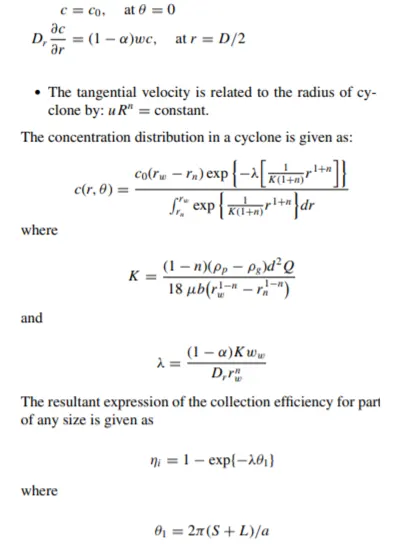
Boundary conditions with the consideration of the turbulent diffusion coefficient and particle bounce re-entrainment on the cyclone wall are:

Koch and Licht model:

Koch and Licht inherently described the turbulent nature of cyclones and distribution of gas residence times within the cyclone. They attributed by the two following assumption:

The tangential velocity of the particle is equal to the tangential velocity of the gas flow. There is no slip in the tangential direction between the gas and particles.

The tangential velocity is related to radius of cyclone by u R^n =constant

Lapple Model –

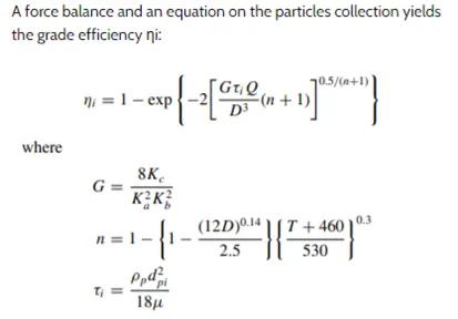
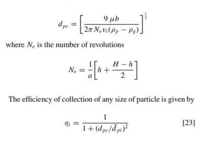
Lapple model was developed based on force balance without considering the flow resistance. Lapple assumed that the particle entering the cyclone are evenly distributed across the inlet opening. The particle that travels from inlet half-width to the wall in the cyclone is collected with 50% efficiency. The semi-empirical relationship developed by Lapple to calculate a 50% cut diameter, dpc is:

Separation Efficiency –

It is defined as the fraction of particles of a given size collected in the cyclone, compared to those of particle sizing going into the cyclone. Model simulation of cyclone separator shows that efficiency increases with:

Increase in -

Particle mean diameter and density;

Gas tangential velocity

Cyclone length

Decrease in –

Cyclone diameter

In our case, we validate the efficiency with particle track history data. Wherein, separation efficiency can be defined as the ratio of concentration that has been removed from the feed steam to initial concentration in the feed steam.

Separation Efficiency = No. of Trapped Particle/No. of Tracked Particle

Pressure Drop –

Pressure drop across the cyclone is much of an importance in cyclone separator. Hence pressure drop significantly affects the performance parameter of cyclone.

Pressure drop is defined as the difference in the total pressure between two points of a fluid carrying network.

`Delta` P = Total Inlet Pressure – Total Outlet Pressure (Escape)

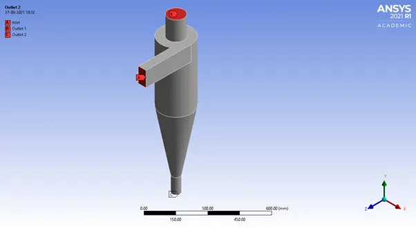
In our case we consider Outlet 1 – Top opening as the DPM -> Escape condition

Procedure –

Problem Setup –

• (1) Geometry

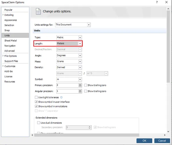
Files → Space Claim Options → Units

Import the geometry and follow the extraction of the model as below –

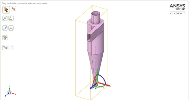
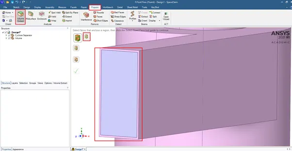
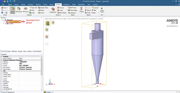
Save the extracted volume as a new design. Just in space-claim doesn’t update with current generated model.

Mesh Generation –

Right Click → Insert → Named Selection, As follows

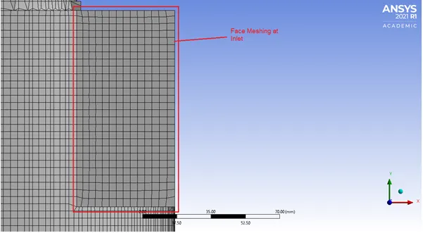
Mesh Setting –

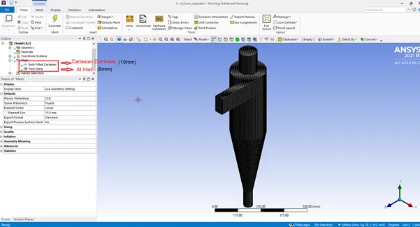
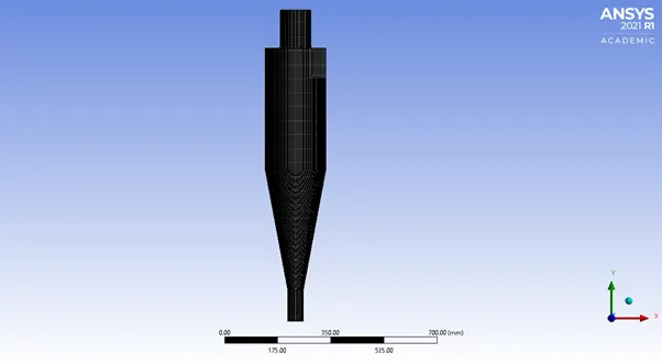
Right Click → Insert → Methods,

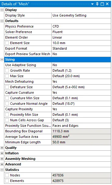
Mesh Details -

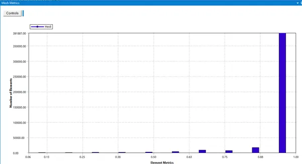
Element Quality –

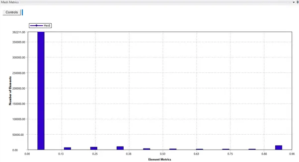
Skewness –

Fluent Setup –

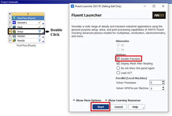
Solution Setup -

• General → Solver → Pressure-based → Time→ Steady State → Gravity → -9.81(y-axis)
• Models → Viscous → RNG → K-epsilon → Swirl dominated flow → SWF
• Discrete Phase →

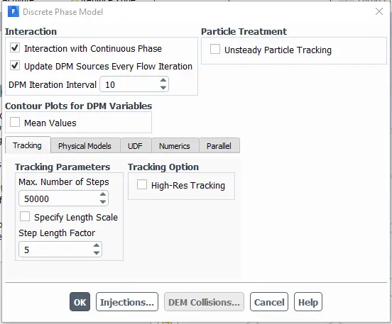
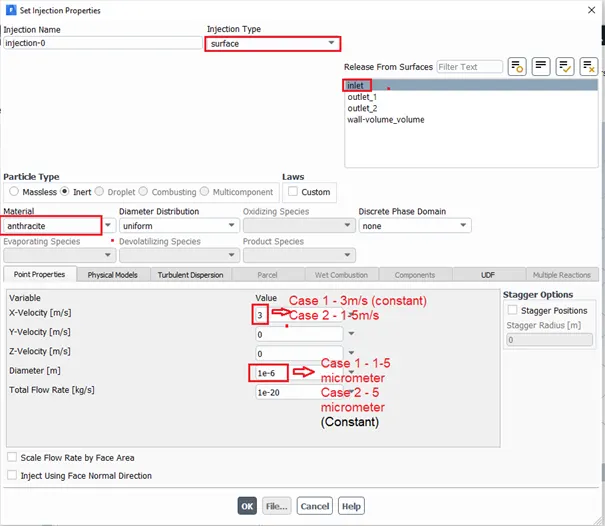
• Boundary Conditions
• Intel (Velocity= Case 1 - 3m/s/ Case 2 – 1-5m/s) → DPM →Reflect
• Outlet 1 (Gauss Pressure=1 atm) → DPM → Escape
• Outlet 2 (Gauss Pressure=1 atm) → DPM → Trap
• Reference Values →

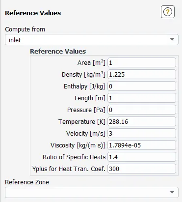
• Method →

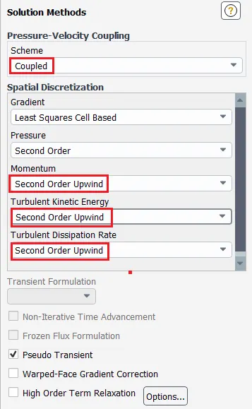
• Results → Create → Point → X(m)= 4 times cylinder diameter → Y(m)= 0
• Initialize Solution → Standard → Compute from inlet
• Results → Export → Particle Track Data → Injection → Write

Results -

Case 1 – Particle diameter size from 1 μm to 5 μm and velocity at inlet = 3m/sec for all sub-cases.

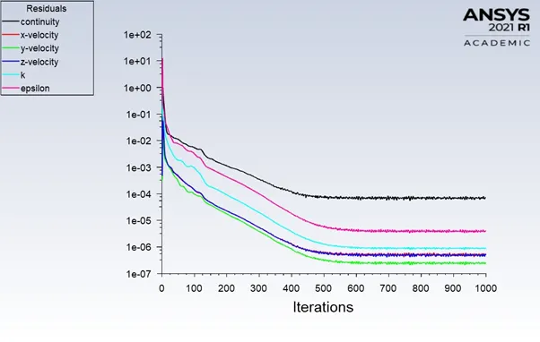
Scaled Residual Plot –

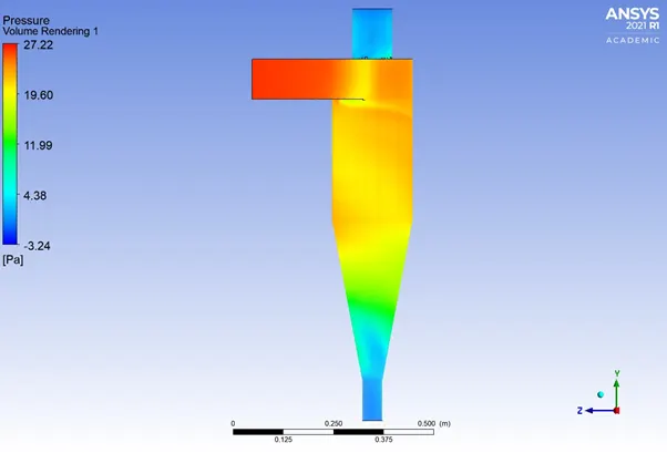
Volume Rendering –

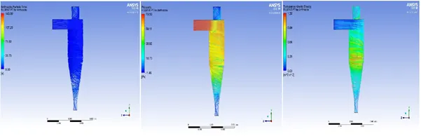
Case 1-a to 1-e –

Case 1-a

Case 2-a

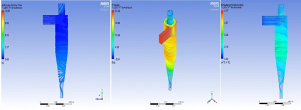
Case 3-a

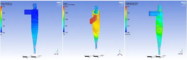
Case 4-a

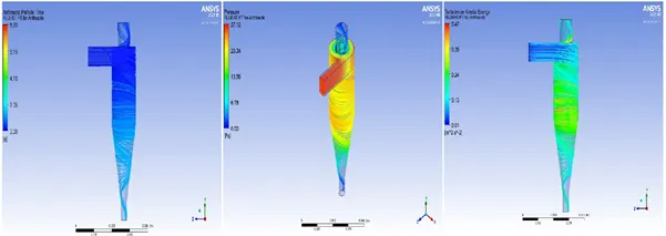
Case 5-a

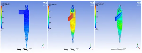
Data Table –

Particle Diameter (m)	Inlet velocity (m/s)	Tracked Particle	Escape Particle	Trapped Particle	Incomplete Particle	Separation Efficiency % = Trapped/Tracked Particles
1e-6	3	378	164	74	140	19.58
2e-6	3	378	102	165	111	43.65
3e-6	3	378	85	203	90	53.70
4e-6	3	378	79	268	31	70.89
5e-6	3	378	16	343	19	90.70

Case 2 –Particle diameter size from 5 μm for all sub-cases and velocity at inlet = 1 m/sec to 5m/sec.

Case 2-a – 2-e –

Case 2-a

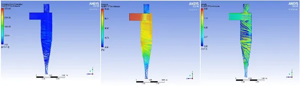
Case 2-b

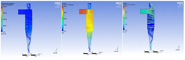
Case 2-c

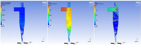
Case 2-d

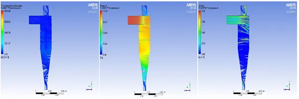
Case 2-e

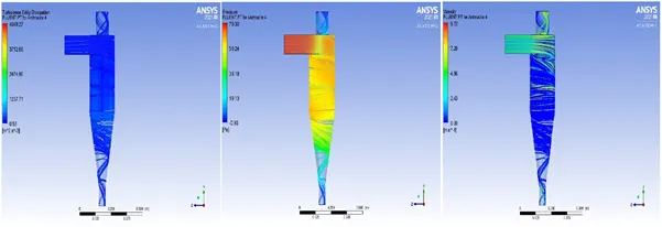
Data Table -

Particle Diameter (m)	Inlet velocity (m/s)	Tracked Particle	Escape Particle	Trapped Particle	Incomplete Particle	Separation Efficiency % = Trapped/Tracked Particles
5e-6	1	378	102	6	270	1.58
5e-6	2	378	75	39	264	10.31
5e-6	3	378	79	282	19	74.60
5e-6	4	378	76	283	17	75
5e-6	5	378	68	310	0	82.01

Conclusion –

• Above pressure plots, infer that pressure is higher near the wall region which in turns forms outer vortex.
• High pressure region near the walls creates a low-pressure area at the centre of cyclone separator because of which the lighter particles tend to escape from the top outlet and heavier particles are collected at the bottom outlet.
• We can observe an energy transfer in form kinetic energy from higher to lighter particle.
• Which results in, certain heavier particles to escape through top outlet and similarly lighter particles get trapped at bottom outlet.
• Collection efficiency of cyclone varies as function of particle size, density and cyclone design.

Cyclone efficiency increase with:

Increase in –

• Particle size
• Density
• Inlet duct Velocity
• Number of gas revolution in cyclone
• Cyclone body length
• Ratio of Cyclone body diameter to Gas exit diameter
• Smoothness of cyclone inner walls

Decrease with increase in parameters as follows –

• Gas viscosity
• Cyclone body diameter
• Gas exit diameter
• Gas density
• Inlet duct area
• Leakages

Total pressure drop occurs due to –

• Entry and Exit losses
• Wall Friction forces
• Rotational kinetic energy
• Swirl and energy dissipation