Week 8 - Simulating Cyclone separator with Discrete Phase Modelling

Aim – To analysis the effective of cyclone separator for the different size of particles for same & differently velocity .

Introduction – The different liquid densities, separating particles from a gas stream by using the equipement is called the cyclone separator . Cyclone separators often form part of a pre-cleaning stage prior to a gas or liquid being discharged. It is also called as dust collector.

Eg : near the exhaust pipe for generators. oil refiner industry for separation of oil & gases.

CYCLONE EFFICIENCY EMPIRICAL MODELS:

1. Iozia and Leith logistic model is a modified version of Barth Model, which work on the force balance. That a particle carried by the vortex endures the influence of two forces: a centrifugal force, Z and a flow resistance, W. The collection efficiency ηi of particle diameter dpi can be calculated from

2. Li and Wang model includes particle bounce or re entrainment and turbulent diffusion at the cyclone wall. A two dimensional analytical expression of particle distribution in the cyclone is obtained.

The following assumptions:

• The radial particle velocity and the radial concentration profile are not constant for uncollected particles within the cyclone.
• Boundary conditions with the consideration of turbulent diffusion coefficient and particle bounce re entrainment on the cyclone wall .
• The tangential velocity is related to the radius of cyclone by: u Rn = constant

Efficiency for particle of any size-

3.Koch and Licht collection theory recognized the inherently turbulent nature of cyclones and the distribution of gas residence times within the cyclone. particle motion in the entry and collection regions with

The following assumptions:

• The tangential velocity of a particle is equal to the tangential velocity of the gas flow, i.e. there is no slip in the tangential direction between the particle and the gas.
• The tangential velocity is related to the radius of cyclone by: u Rn = constant

1. Lapple model -This force balance without considering the flow resistance. Assuming the particle entering the cyclone is evenly distributed across the inlet opening. The particle that travels from inlet half width to the wall in the cyclone is collected with 50% efficiency. The semi empirical relationship developed by Lapple to calculate a 50% cut diameter, dpc, is

The efficiency of collection of any size of particle

Solving & Modelling approach-

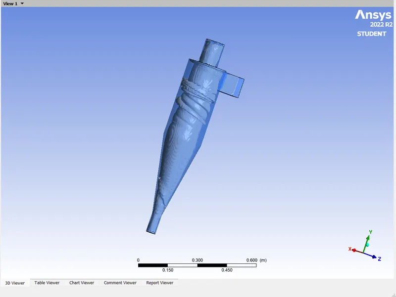
After opening the space claim import the cyclone separator model in to it.the extrac the fluid volume by using the extract tool.then supress the model.

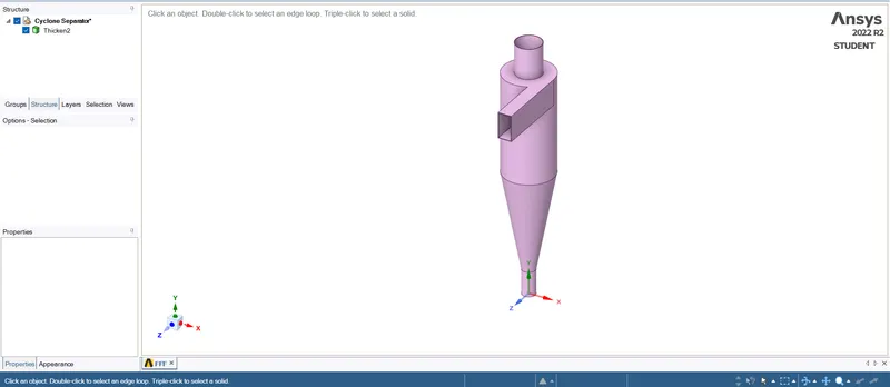
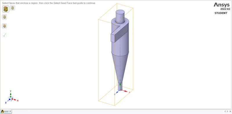
Geometry & fluid volume.

Pre-processing and solver setting-

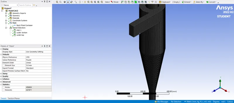
Meshing & naming.

Setup

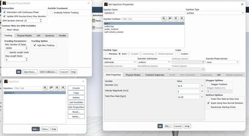
Applying the boundary conditions, solution methods ,plots ,viscous models & DPM to the geometry.

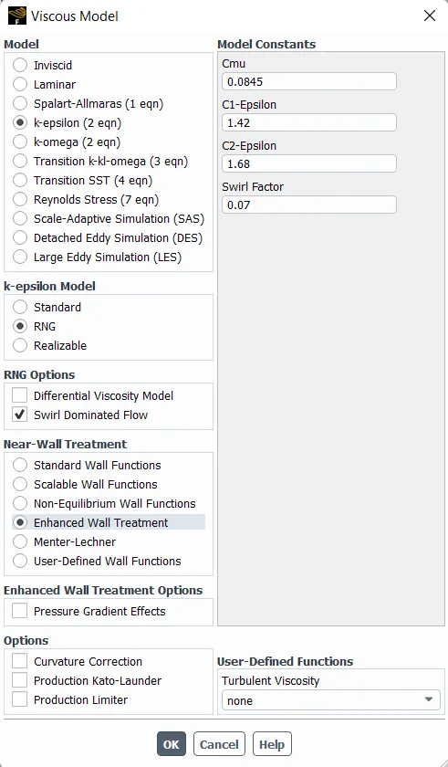
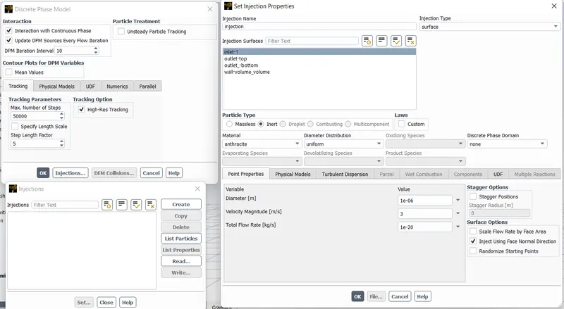
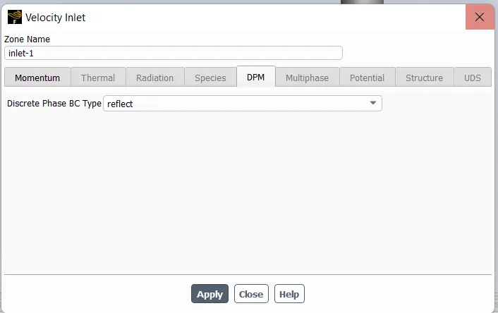
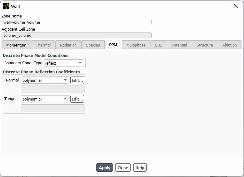
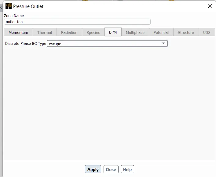
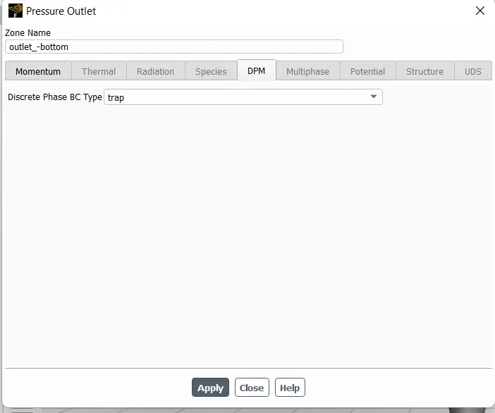
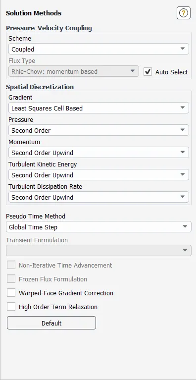
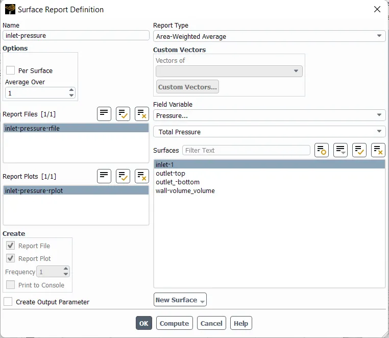
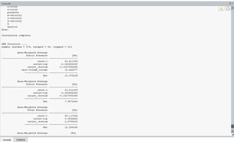
for 1 mm particles results for 3m/s.

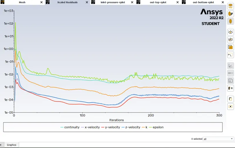
residuals

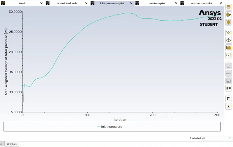
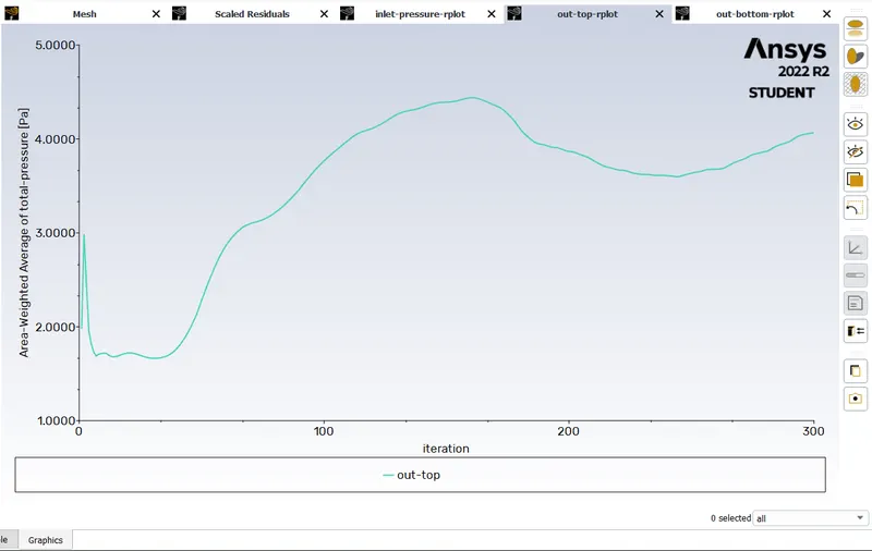
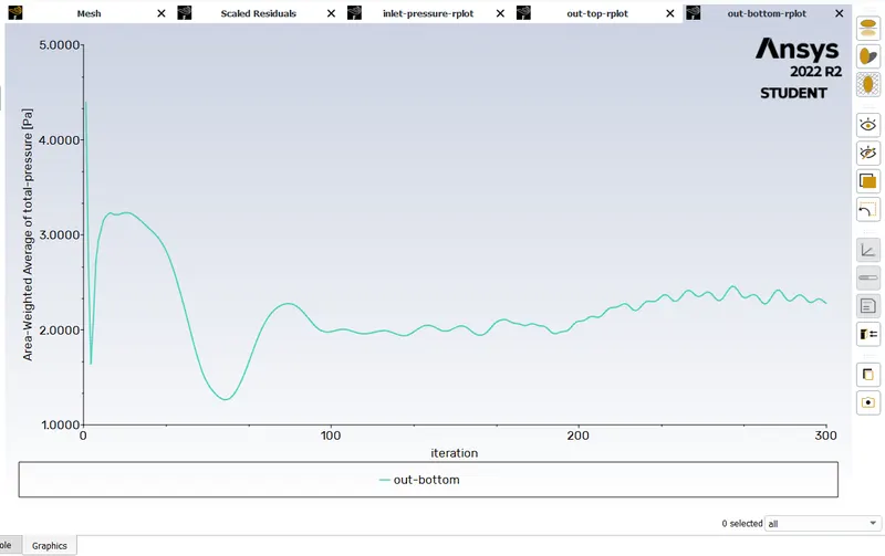
pressure drops for inlets &outlets.

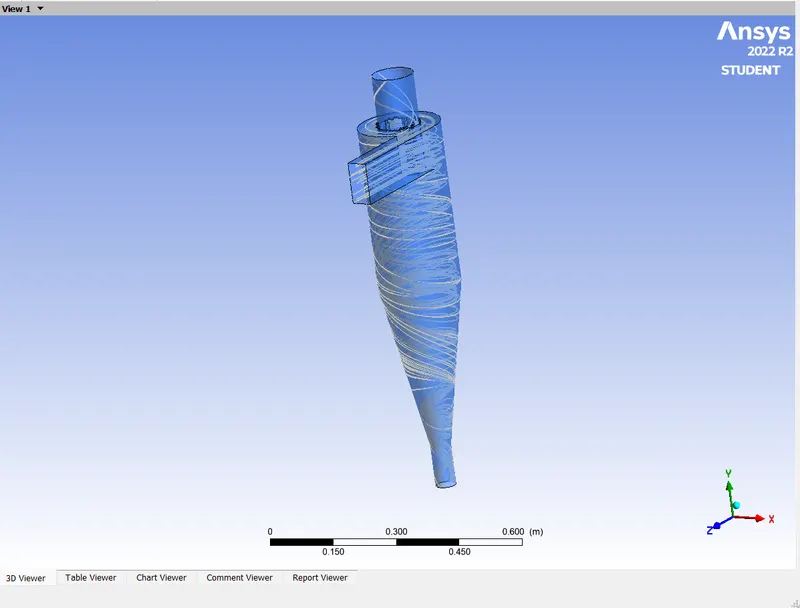
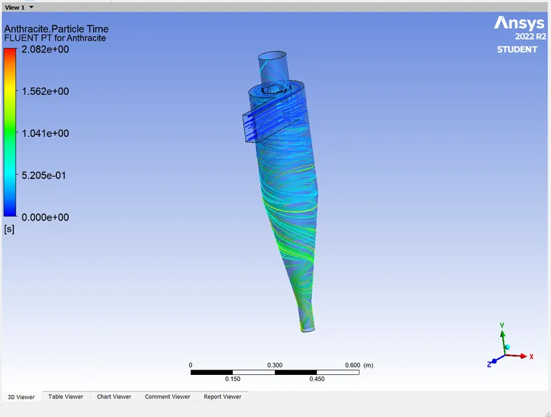
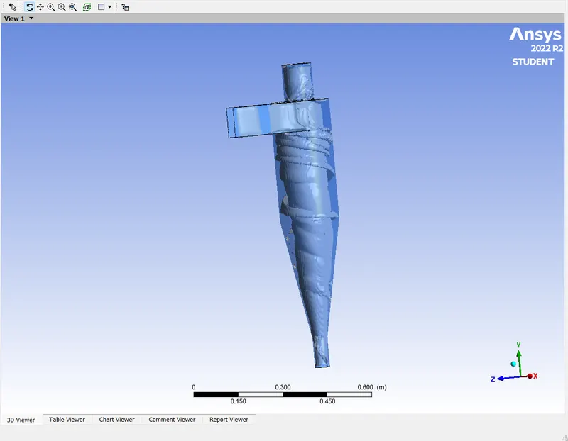
contours ,vertex results.

animation link - https://drive.google.com/file/d/1wySO-d09WP5Yqo8Uzv9pkg0lIjKNtAvj/view?usp=drive_link

for 2mm particles results for 3m/s .

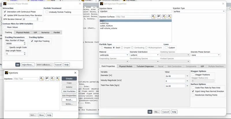
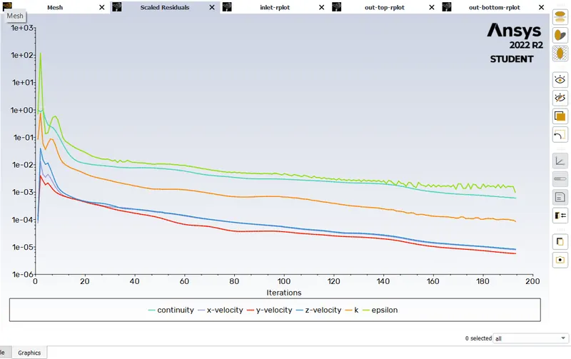
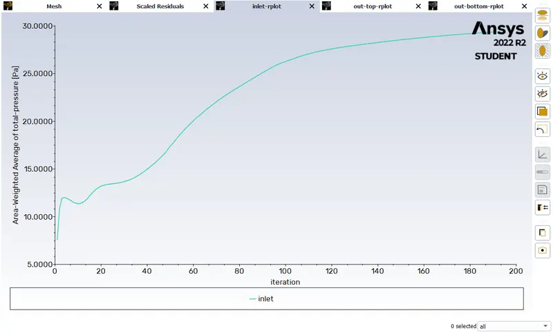
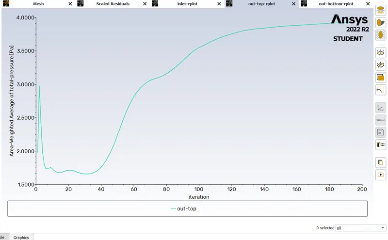
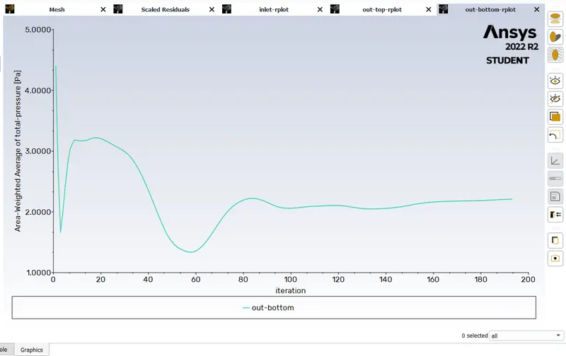
residuals,pressure plots results

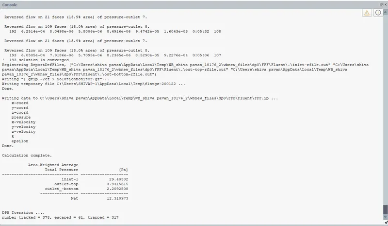
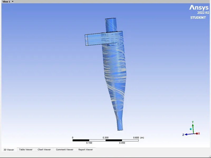
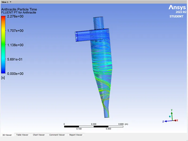
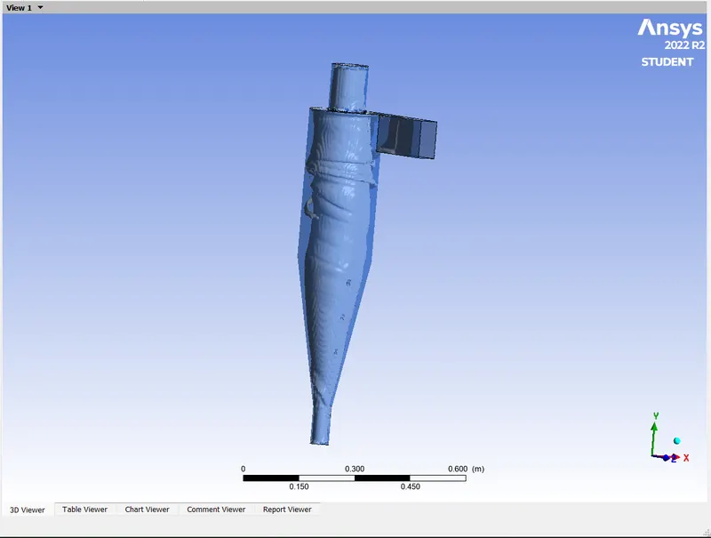
contours ,vertex results

Animation links- https://drive.google.com/file/d/1-NgOHm-bqjeFDKfMzqjdAx0_L10Y95fn/view?usp=drive_link

for 3mm particles results for 3m/s .

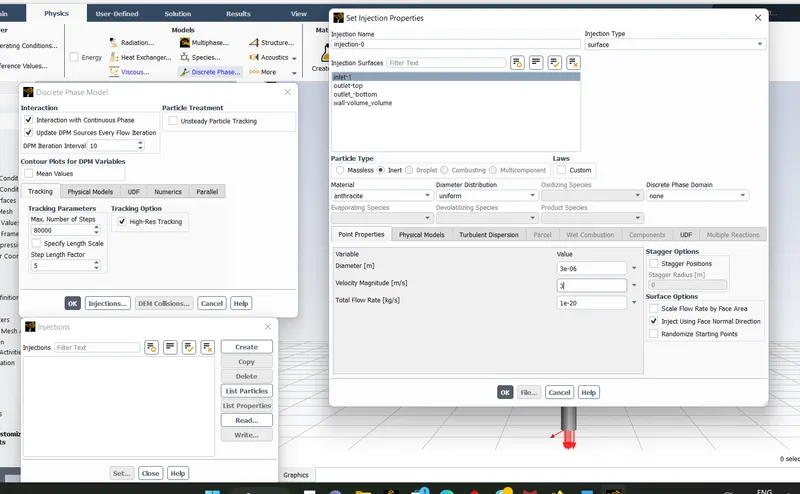
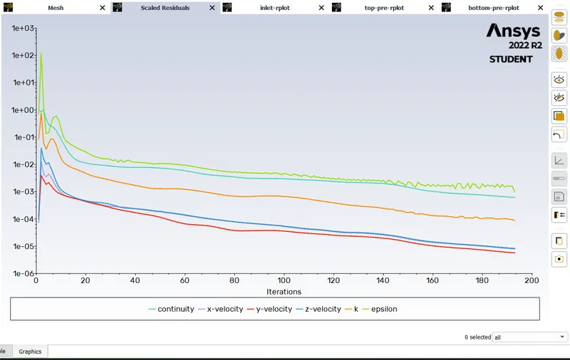
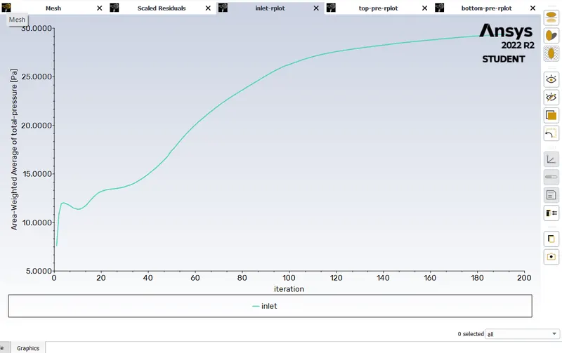
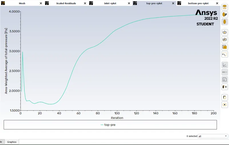
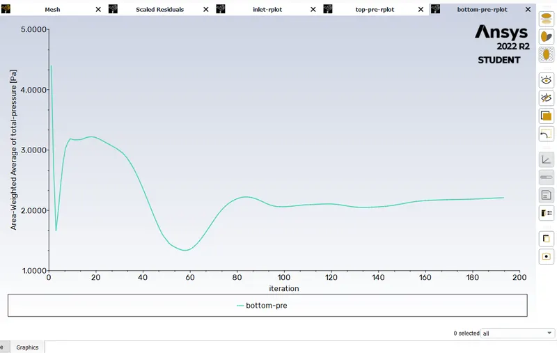
residuals, pressure plot results.

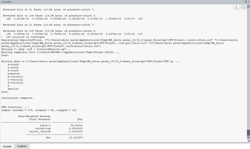
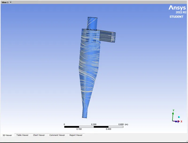
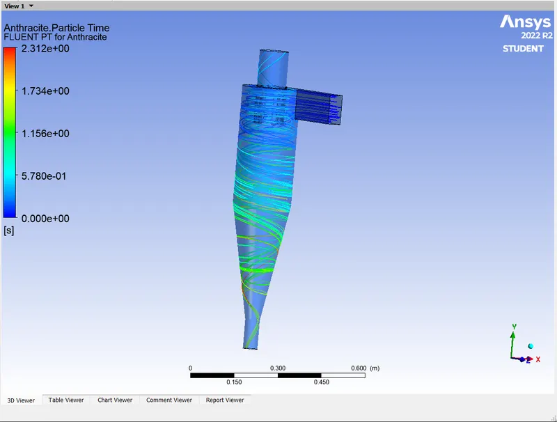
contours,vertex results.

Animation link- https://drive.google.com/file/d/1aKkJNIPmumM2q5A4-O-N6z-Eu0wPqJCQ/view?usp=drive_link

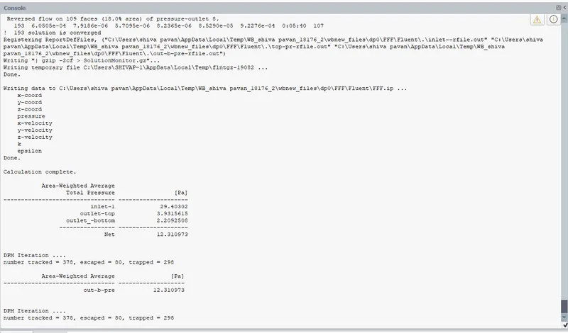
for 4mm particles results for 3m/s .

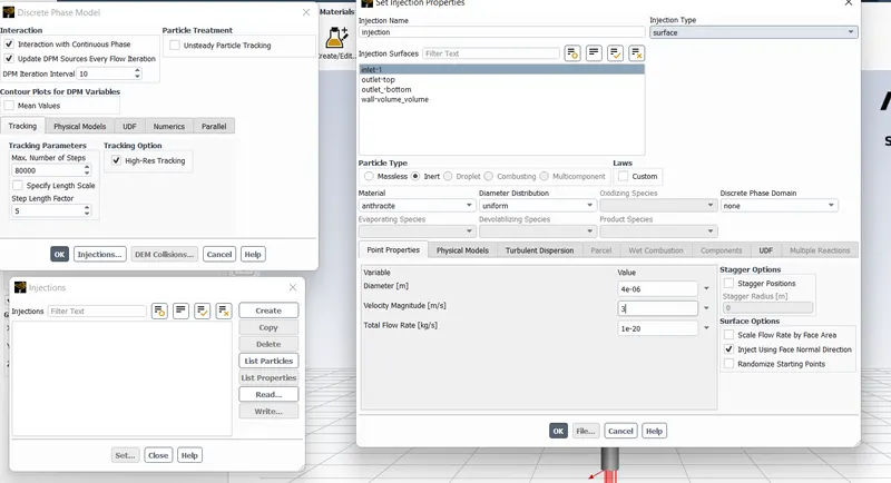
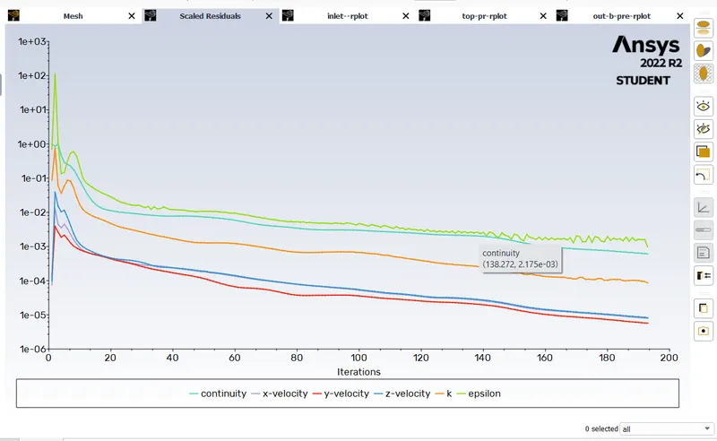
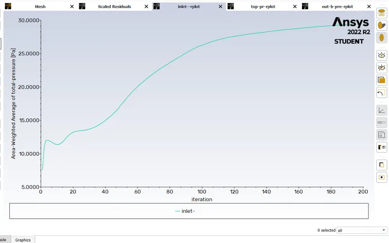
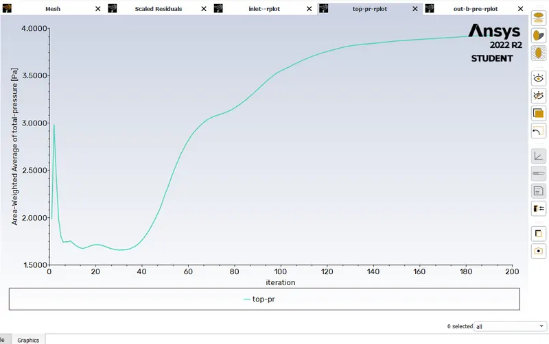
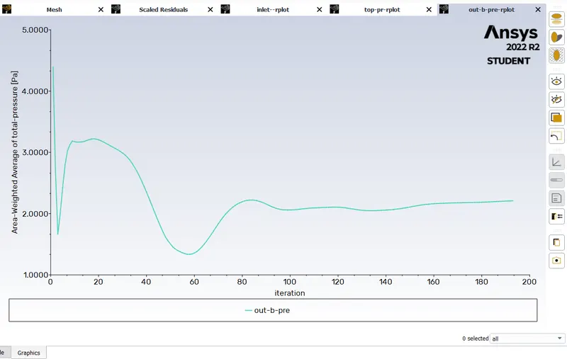
residuals,pressure plots results

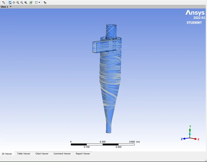
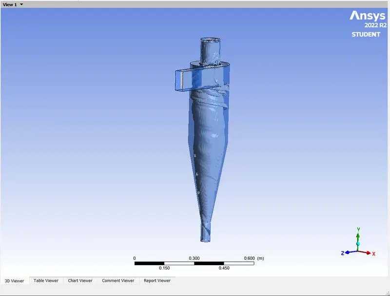
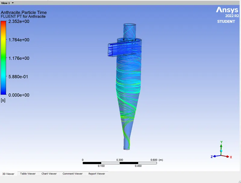
countour , vertex results

Animation link- https://drive.google.com/file/d/1FO-jLY03VifZdvSmy1A2rTveUCE9gJN4/view?usp=drive_link

for 5 mm particles results for 3m/s .

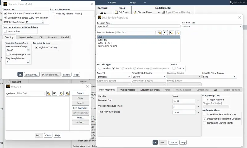
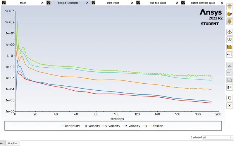
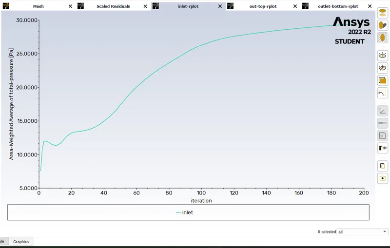
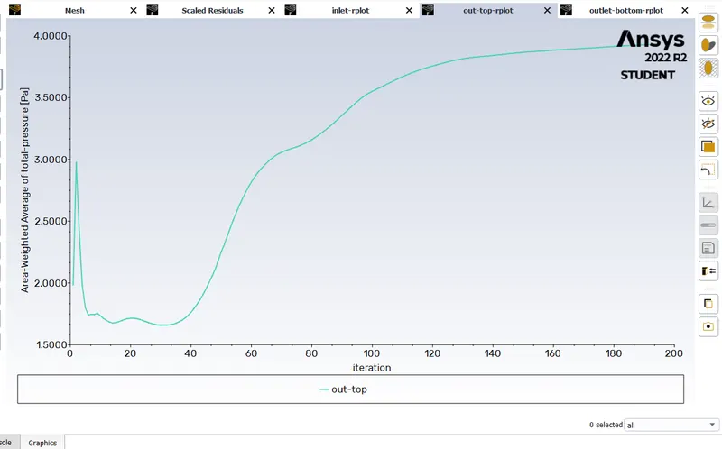
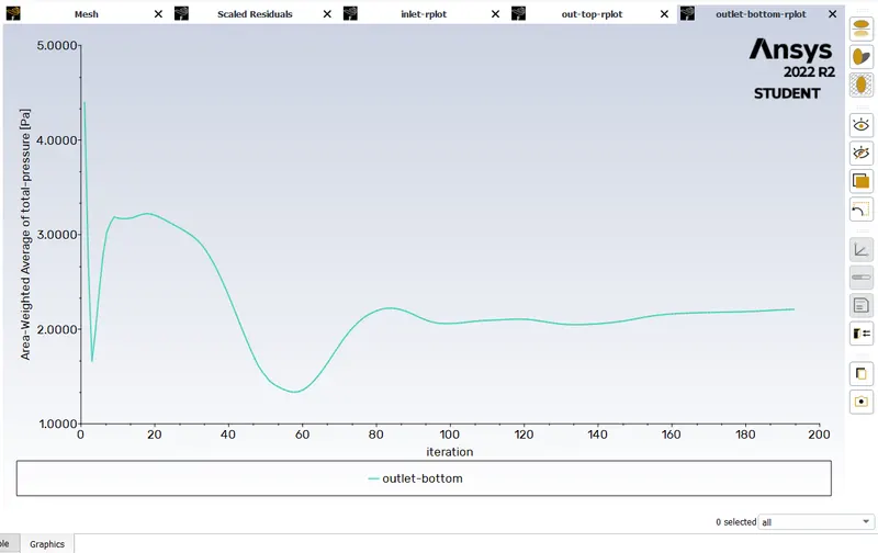
residuals,pressure plots.

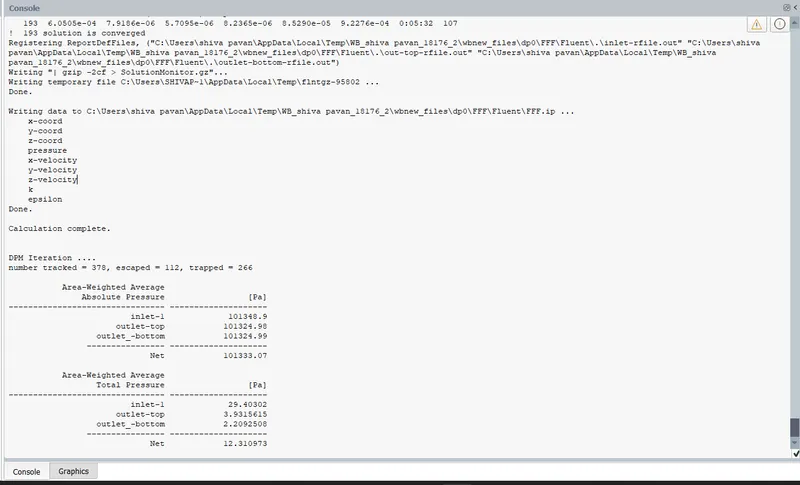
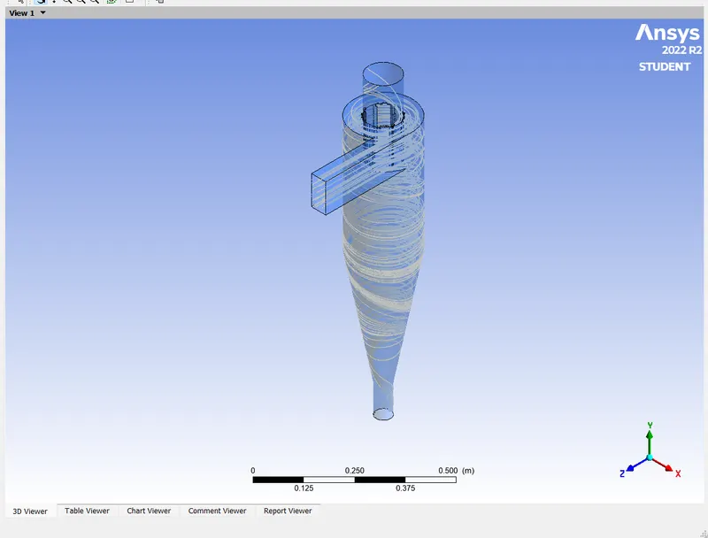
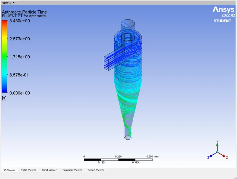
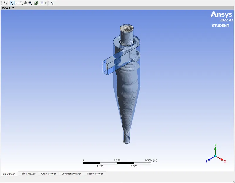
vertex ,contour results.

Animation link - https://drive.google.com/file/d/1OLnuAXbsQbIUW5UDO8hBYZjrXFXHRbG4/view?usp=drive_link

Below table for the efficiency for constant velocity for different sizes of particales.

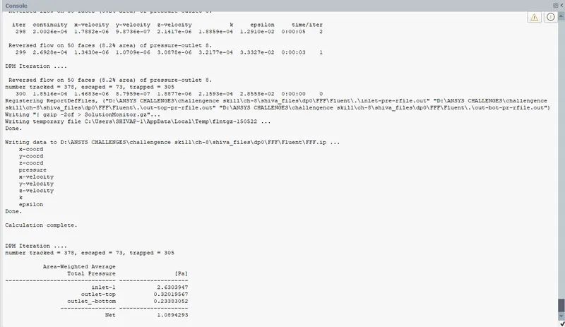
for 1mm particle size , 1m/s velocity

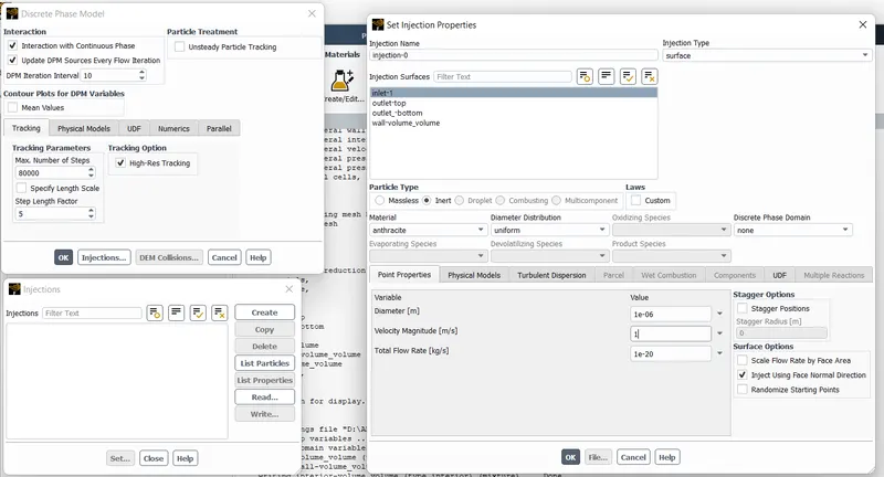
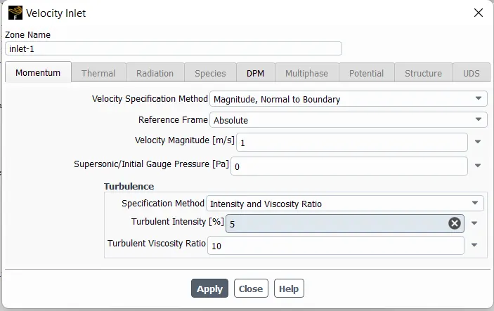
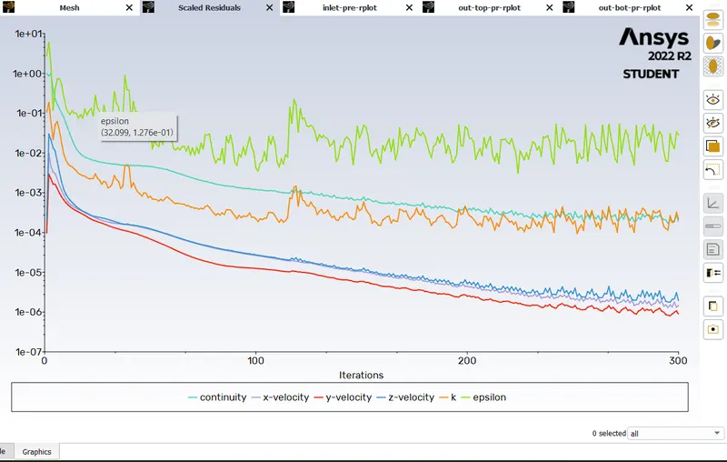
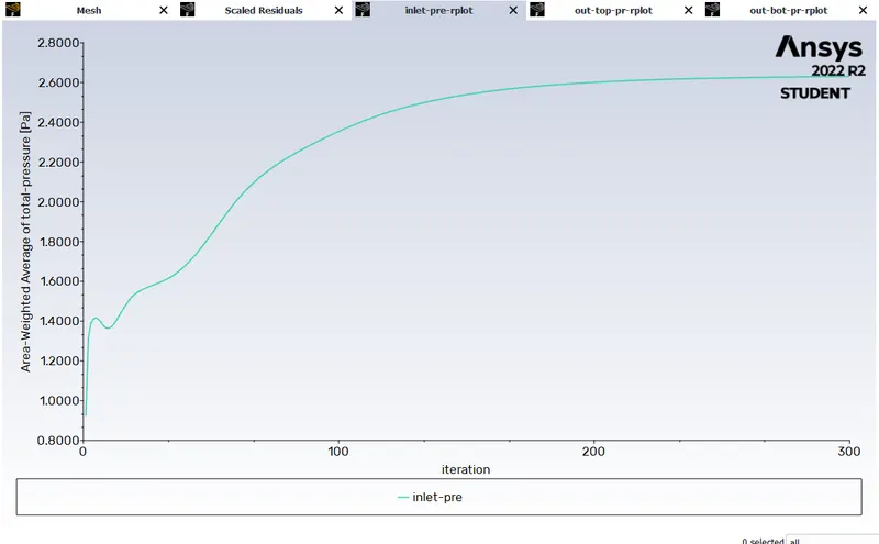
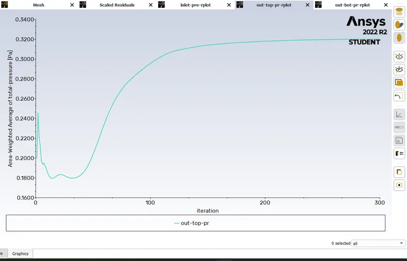
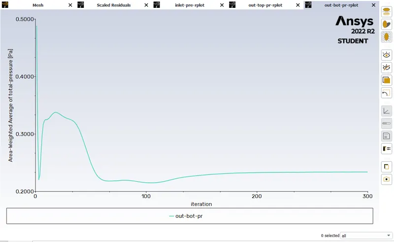
residuals ,pressure plots.

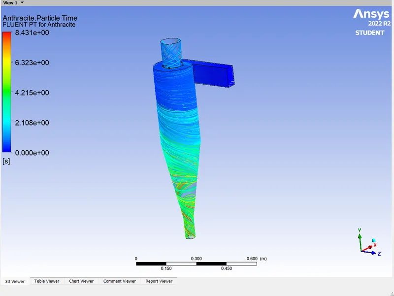
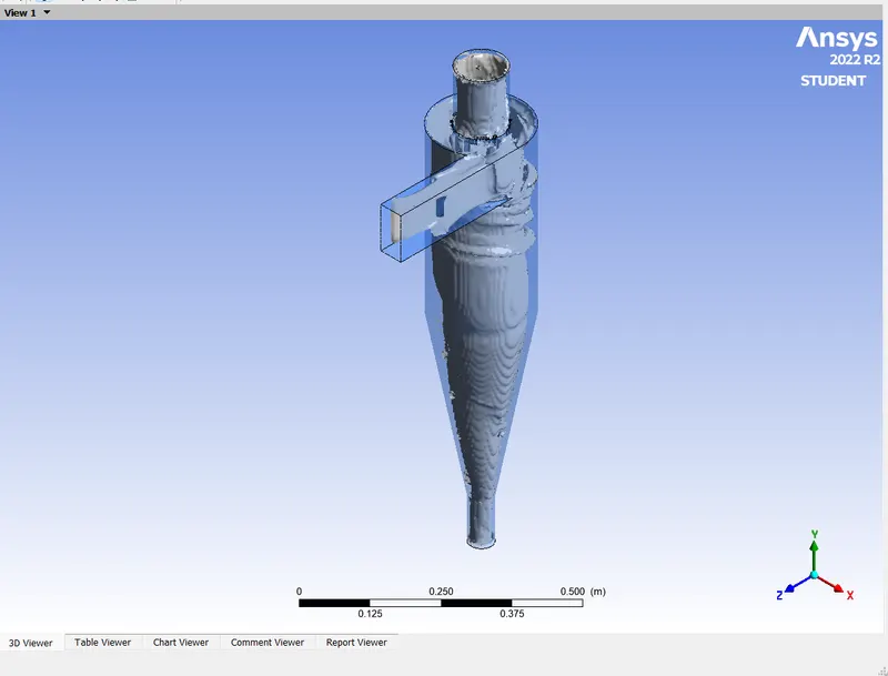
vertex,contour plots.

Animation links- https://drive.google.com/file/d/17Ob-ZttL-f7yOn_xJ97va2Il-Eu9gAtd/view?usp=drive_link

for 2 mm particle size , 2 m/s velocity

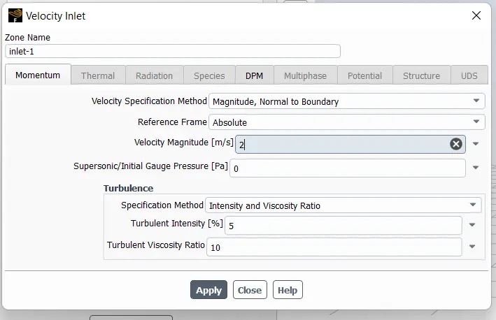
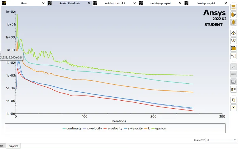
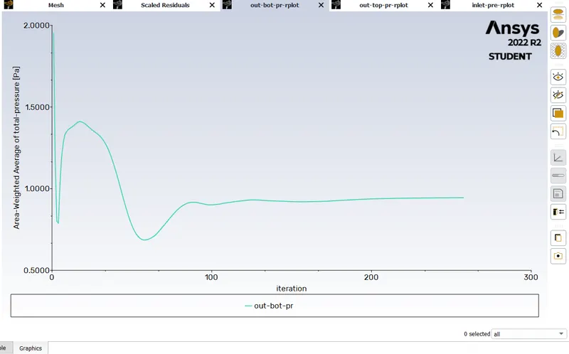
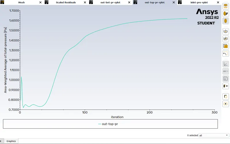
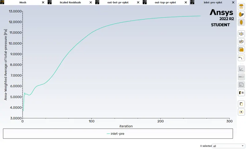
residuals,pressure plots

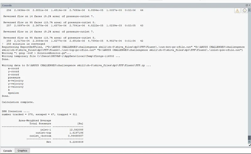
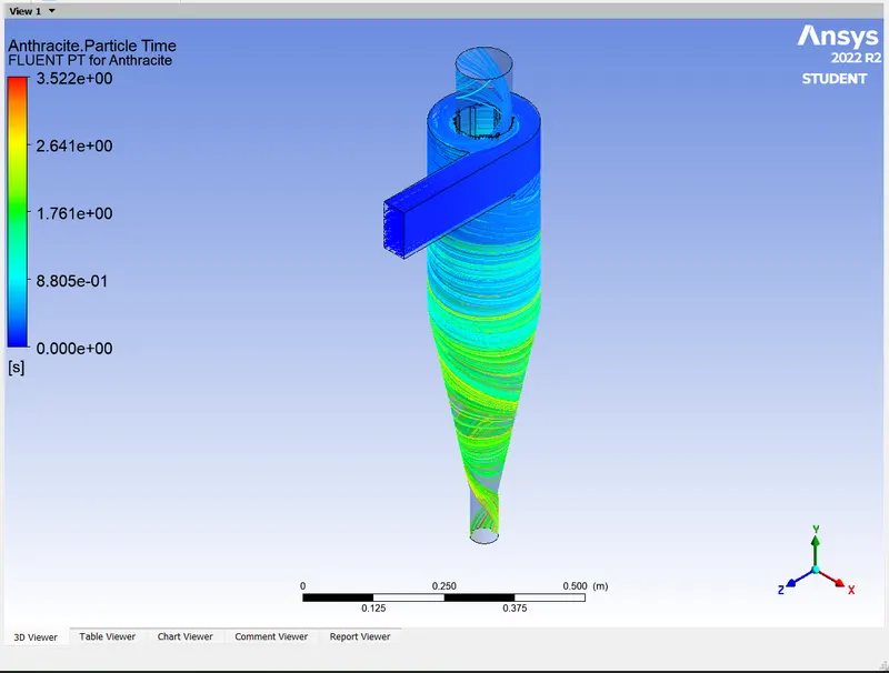
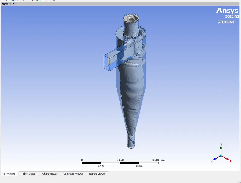
contour,vertex

Animation link - https://drive.google.com/file/d/1NA3oeYi_ZMsRcxtz4sThCuIqi8WdtbMG/view?usp=drive_link

for 3 mm particle size , 3 m/s velocity

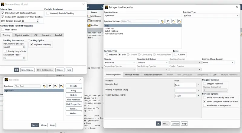
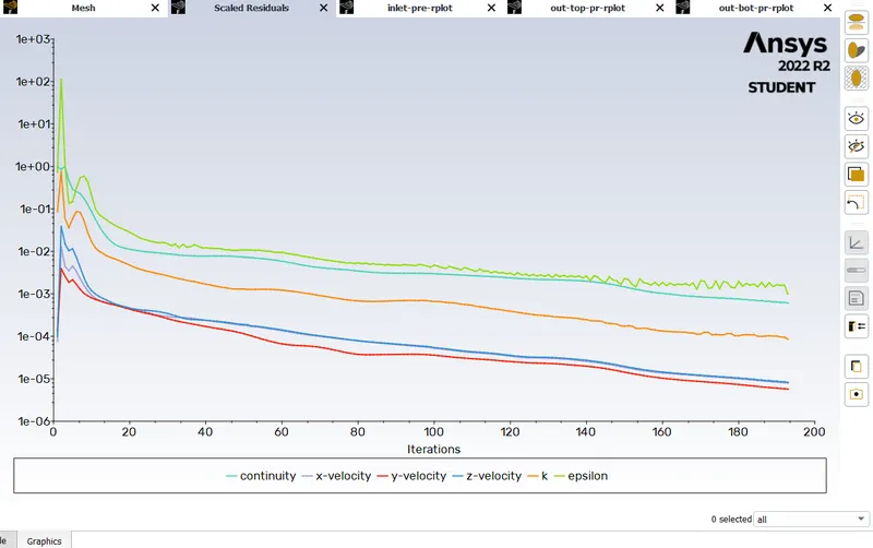
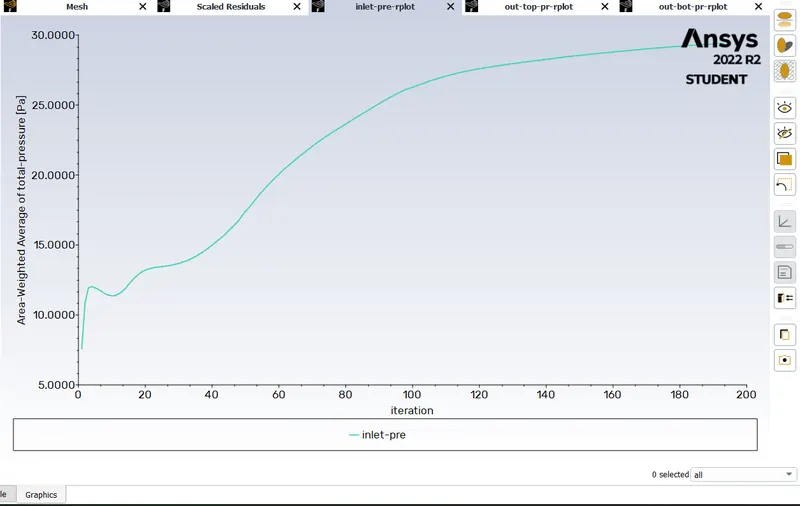
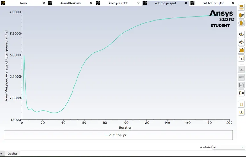
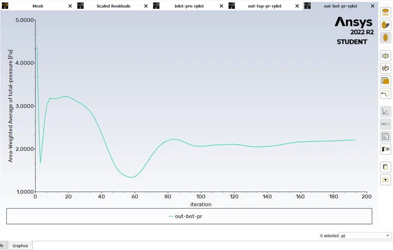
residuals, pressure plots

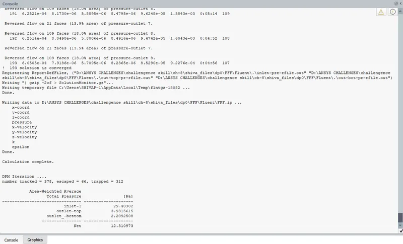
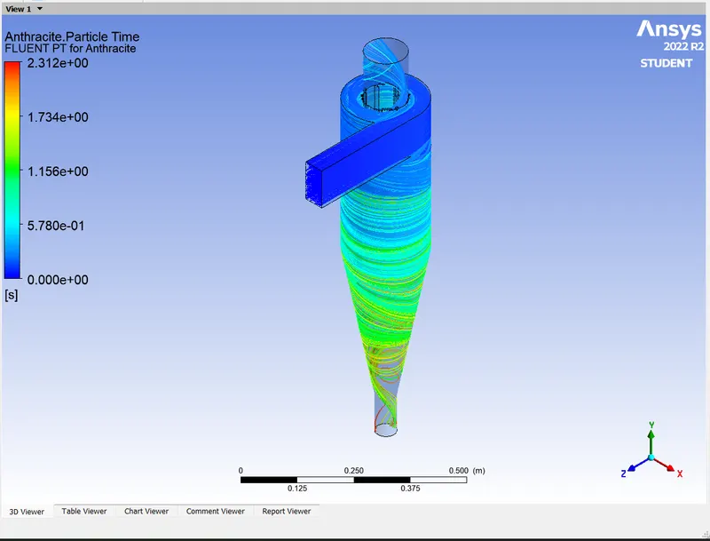
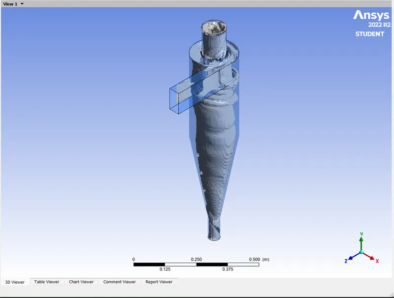
Vertex,contour results.

Animation link- https://drive.google.com/file/d/13cO4gdjkW73L2dnSKNjIF3DLYK5-8JAg/view?usp=drive_link

for 4 mm particle size , 4 m/s velocity

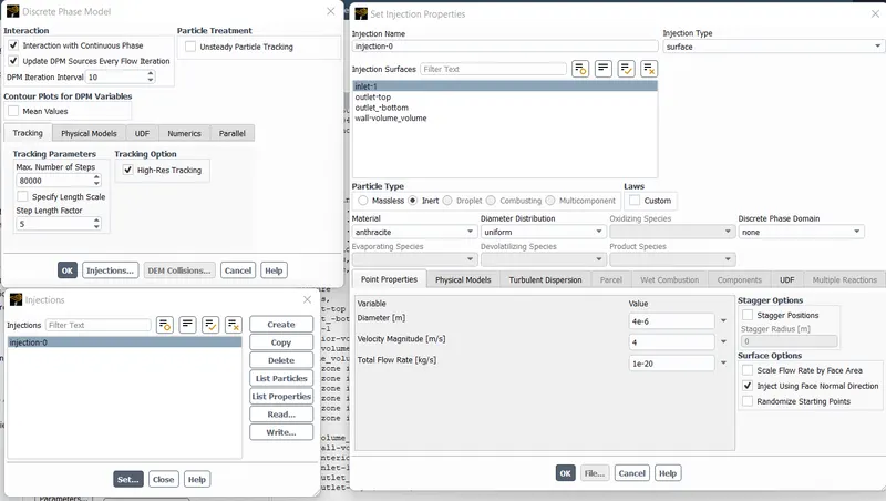
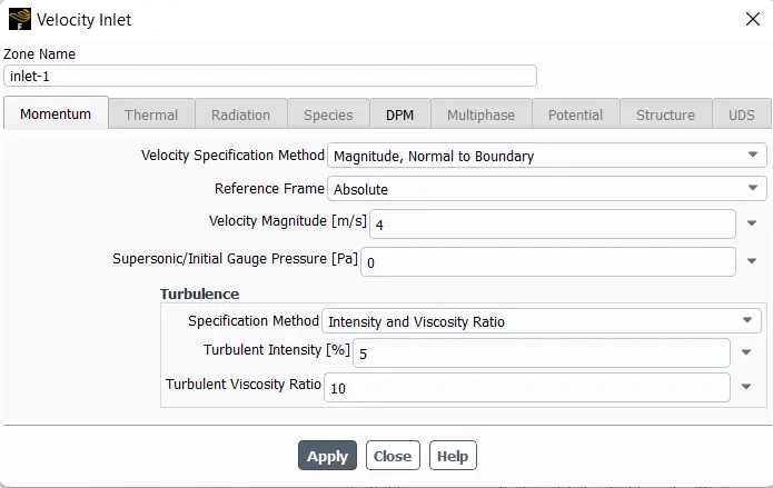
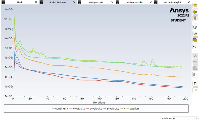
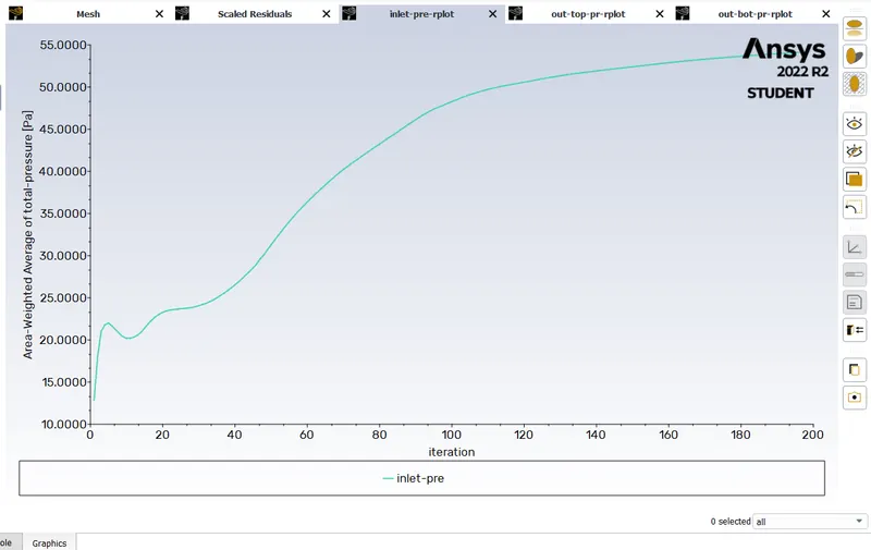
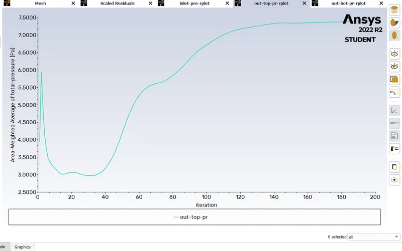
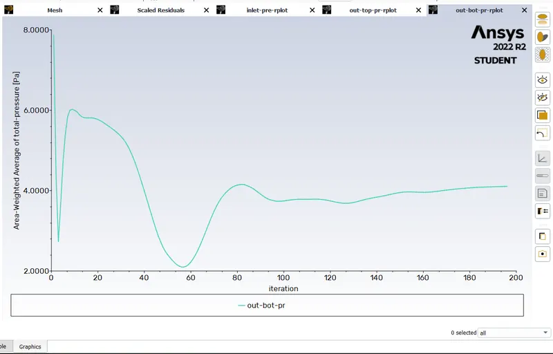
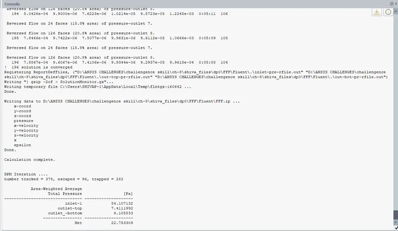
residuals,pressure plots.

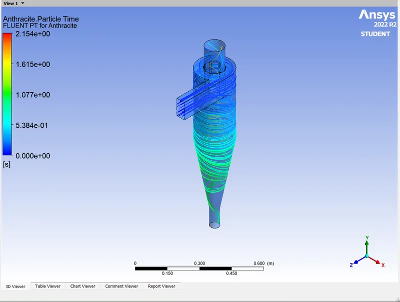
contour,vertex results

Animation links - https://drive.google.com/file/d/1Po0P1NUh6V0qtpkgiu-9FUdF_rLHSENN/view?usp=drive_link

for 5 mm particle size , 5 m/s velocity

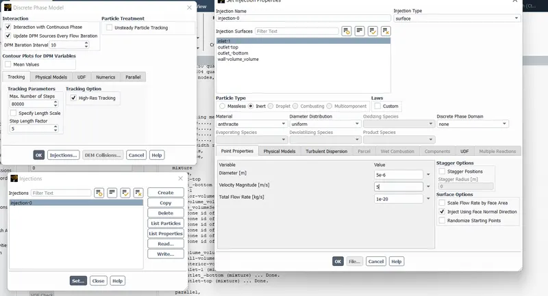
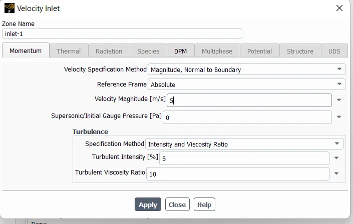
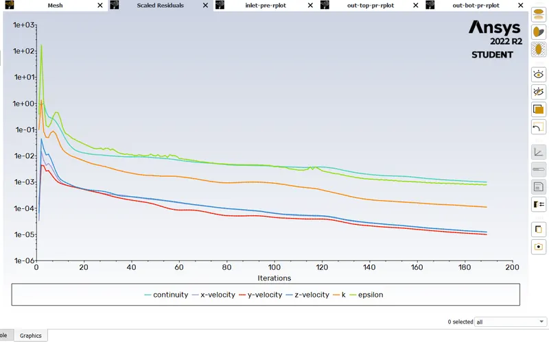
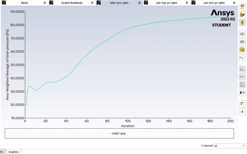
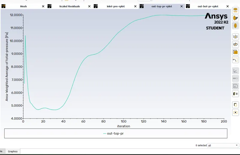
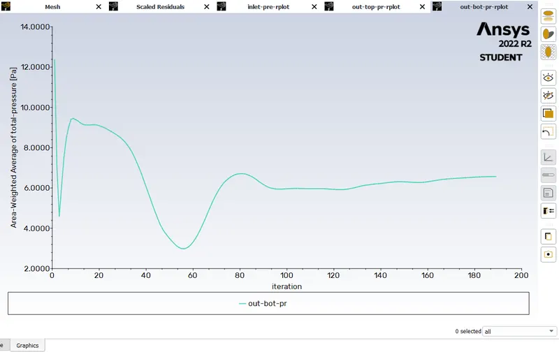
residuals,pressure plots

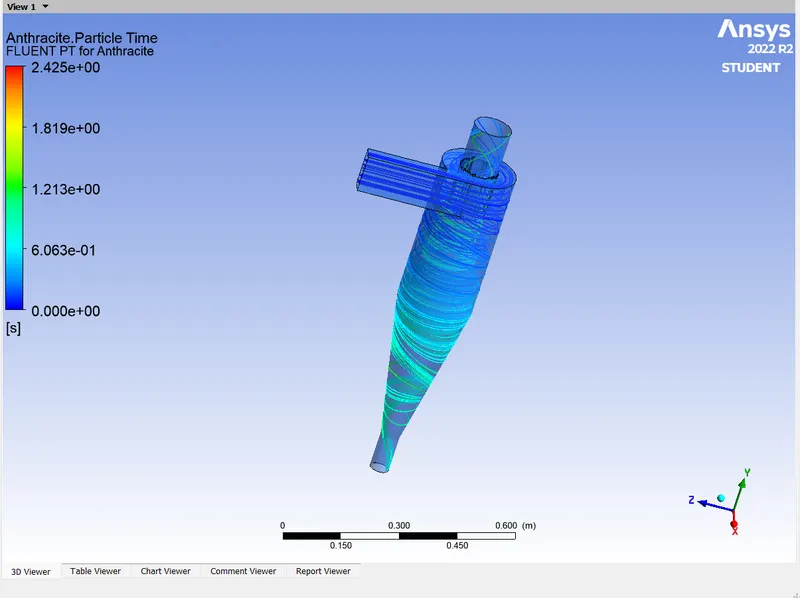
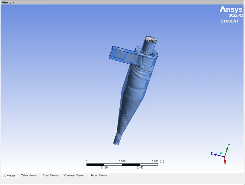
countour ,vertex results.

Animation link- https://drive.google.com/file/d/1lxE1Bzaooh70ioU7pjp44KoxLW-OUPqI/view?usp=drive_link

Below table for same size particles as same velocity results.

conclusion-

Separation efficiency depends on both the diameter and velocity of the particles. As increased diameter and velocity gives increased separation efficiency.

pressure drop is increasing can see as the velocity is increased.

For constant velocity with varying diameter sizes, the pressure drop remains almost constant.