Week 2 - Flow over a Cylinder.
Aim: To get the flow vortex for the cylinder at the different Reynolds numbers and get the Coefficient of drag ,Coefficient of lift .
INTRODUCTION:-
The phenomenon of Karman vortex street is a repeated pattern of vortex shedding after the body . we will see the flow separation from the body. Behaviour of the different fluids can change for the different parameters like viscosity, Reynolds number, density etc. practical application are the flow over the aerofoils structures, wind mills , tall towers, chimneys , Tall buildings etc.
Solving & Modelling approach
Creating the geometry for the flow over cylinder . By the taking the circle from sketch group tab. Drawing the circle 2 mts diameter at the coordinator center. Then by taking the construction lines of 20mts & 10mts from the center of circle. the horizontal ,vertical lines are drawn as a reference for rectangle boundary for simulation. Generating the rectangle by measurements of 20mts * 60mts taking the construction lines as the reference. Deleting the construction line from the structure tree. making the plane for simulation by using the pull tool . we need to change the units from MM to METERS before the starting the geometry.
Generating the model in space clam :
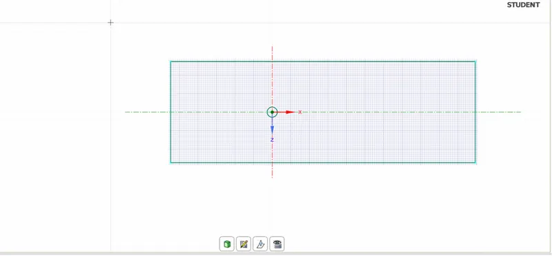
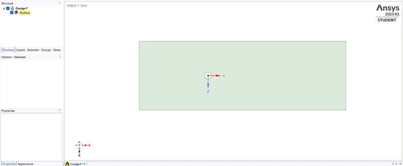
Generating the mesh for the geometry: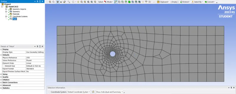
Created the primary mesh for geometry . inserting the method mesh
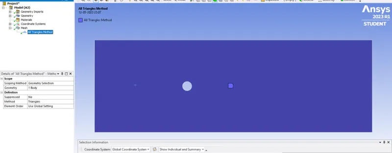
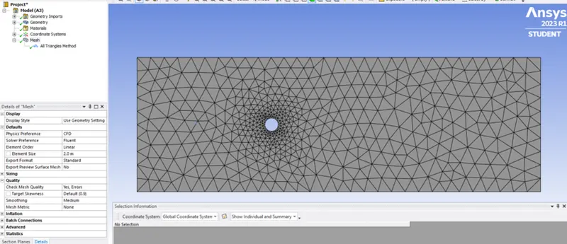
Changing the quadrilateral mesh to triangle mesh by inserting the method mesh and giving the 2m mesh size .
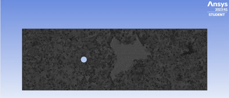
Refined the mesh from 2mts to 0.25mts.
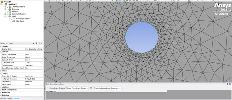
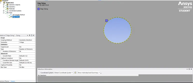 Making the cylinder more smooth for the fine mesh.
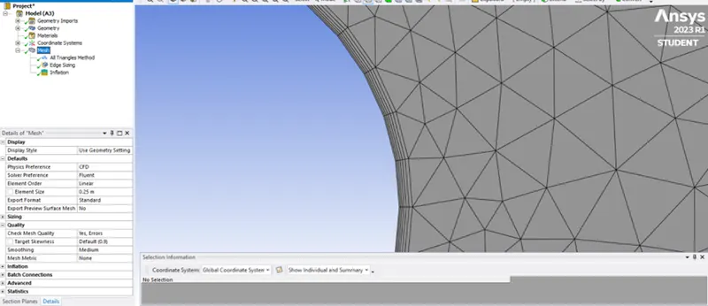
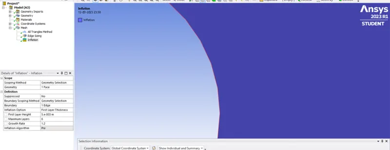
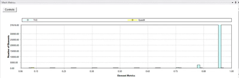
Applying the inflation layers to the cylinder & checking the mesh quality.
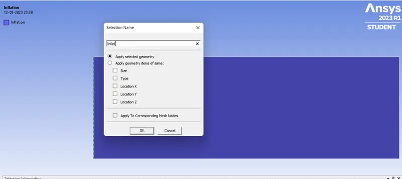
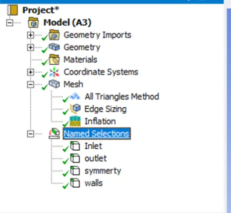
Creating the name to the boundaries -inlet, outlet, symmetry ,cylinder walls.
Pre-processing and solver setting
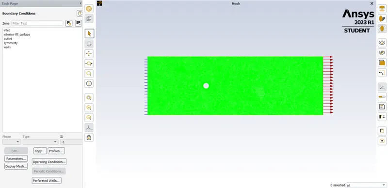
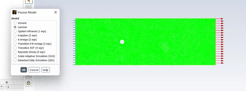
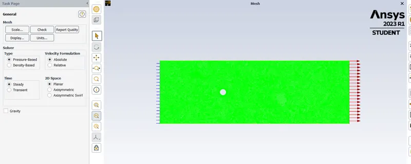
Setting the flow as a laminar flow
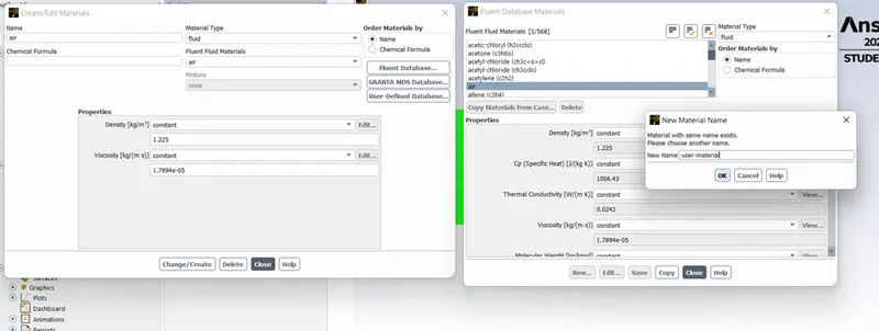
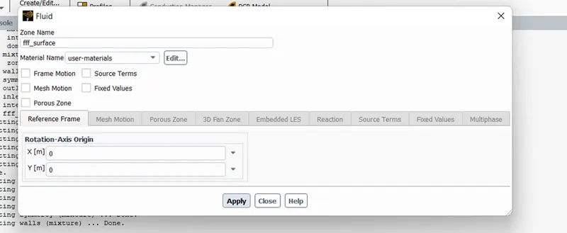
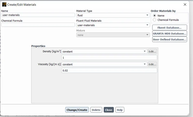 creating the new material for geomerty
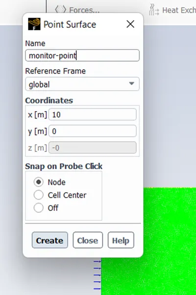
creating the monitor point
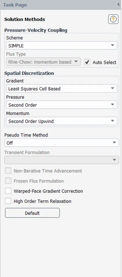
changing the couplied to simple for solution
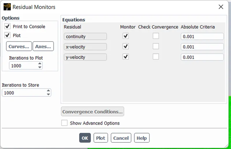
changing the uncheck for convergence
Creating the plots , contours, animations for geometry
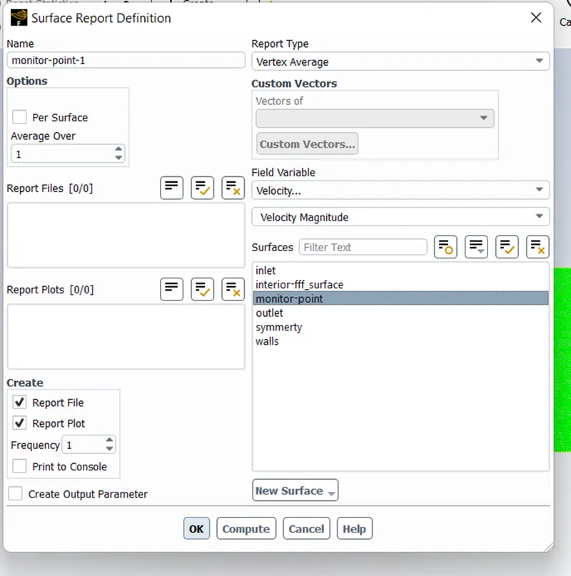
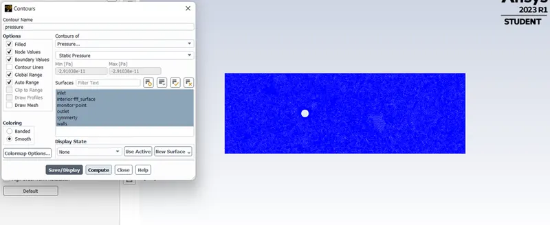
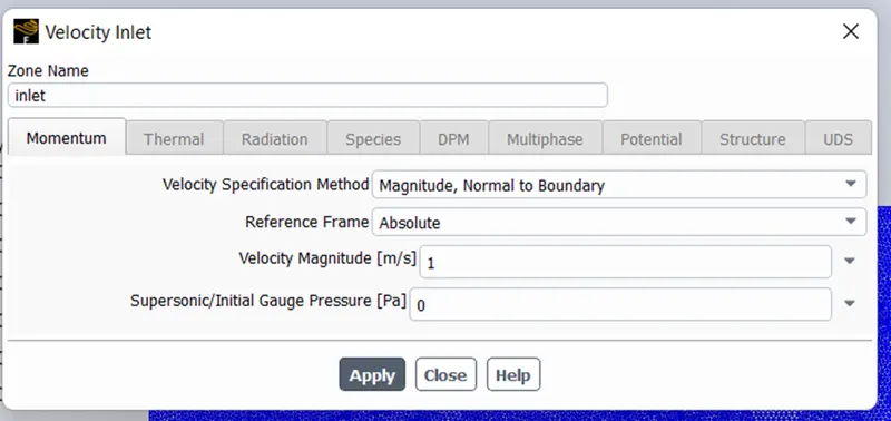
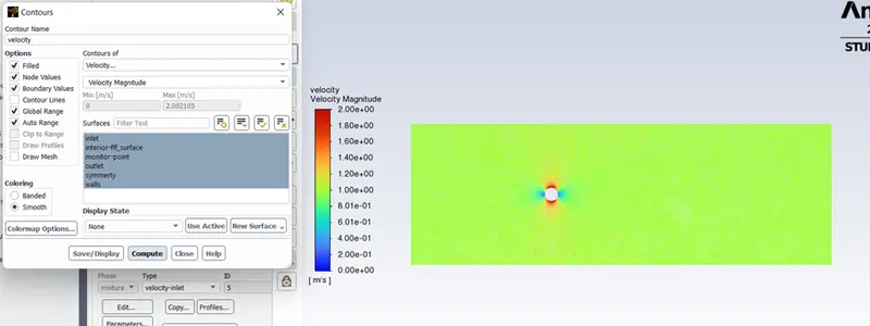
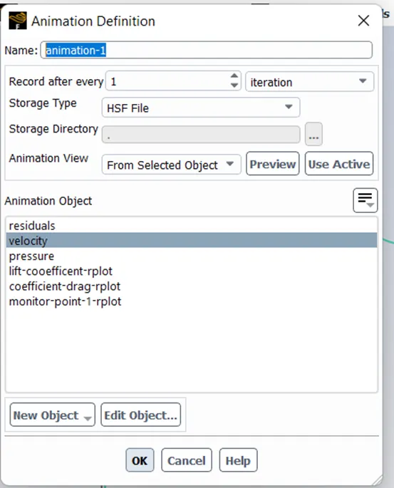
Reynolds no-10
Steady flow
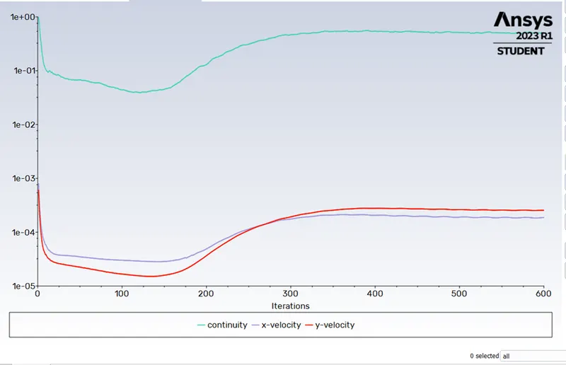
Residual plots
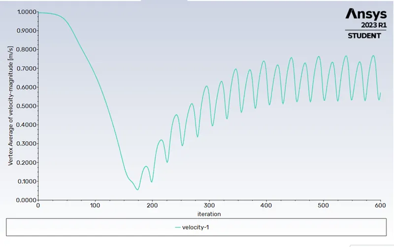
Vertex avg velocity
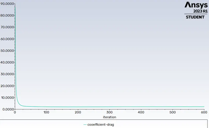
Coefficient of drag
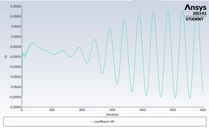 Coefficient of lift
contours plots-
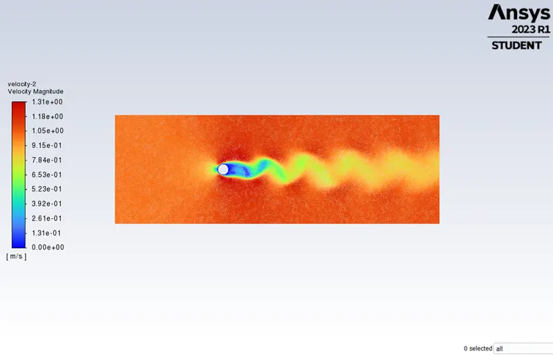
Velocity
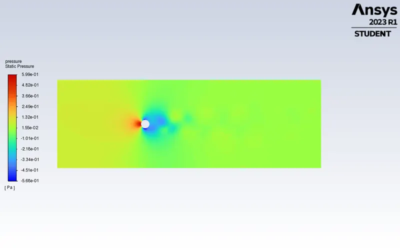 pressure
Unsteady flow
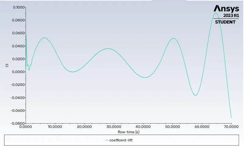
Coefficient of lift
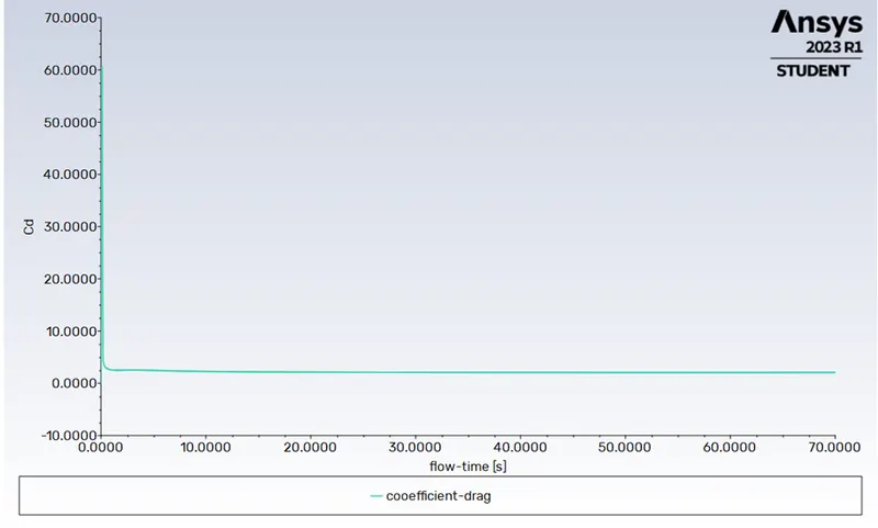 Coefficient of drag
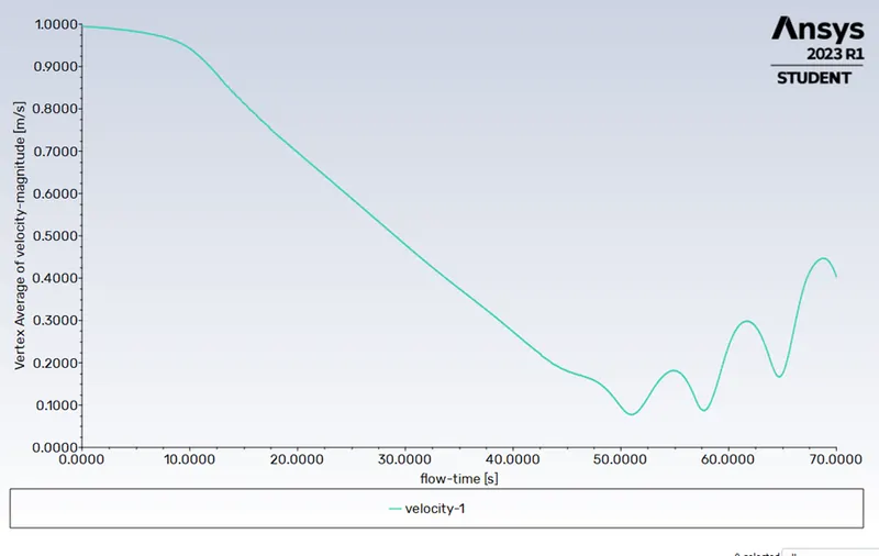
Vertex velocity
Contours plots
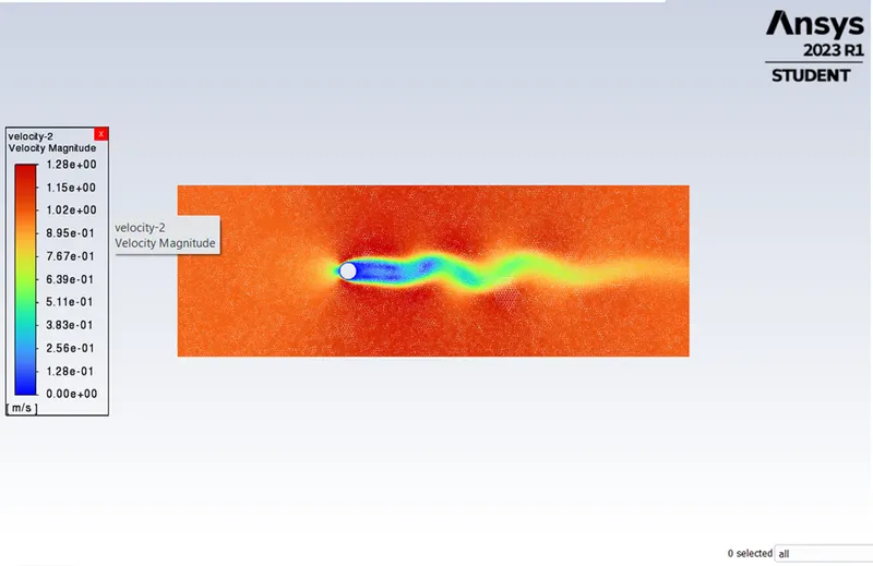
velocity
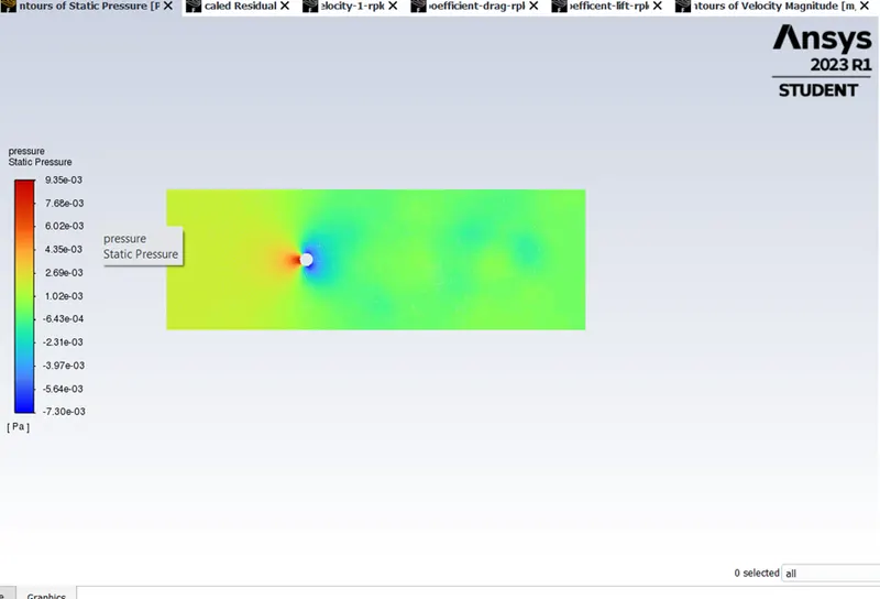
pressure
R e = ρ V L/ μ
Reynolds no- ρ = density, u = velocity, D = diameter, μ = absolute viscosity
|
Reynolds no |
velocity |
Viscosity |
density |
Iterations |
|
10 |
0.1 |
0.02 |
1 |
300 |
|
100 |
1 |
0.02 |
1 |
300 |
|
1000 |
10 |
0.02 |
1 |
300 |
|
10000 |
100 |
0.02 |
1 |
300 |
|
100000 |
1000 |
0.02 |
1 |
300 |
Reynolds no-10
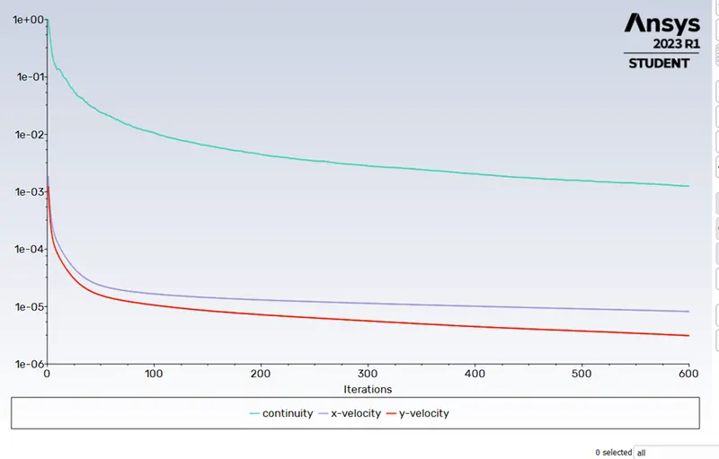
Residual plots
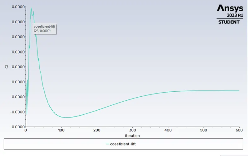
Coefficient of lift
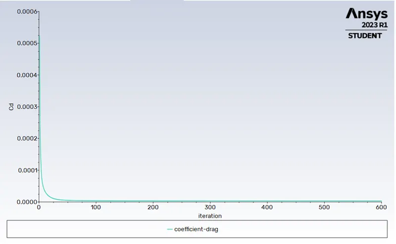
Coefficient of drag
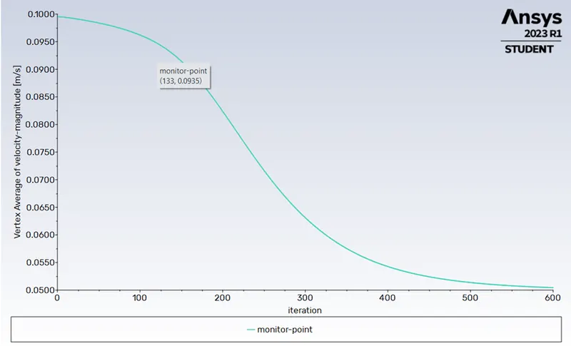
Vertex velocity at monitor point
Contours plots-
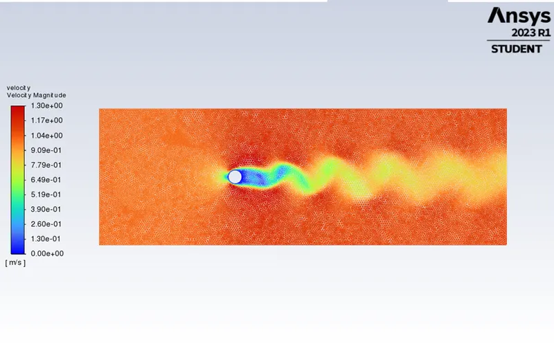
Velocity
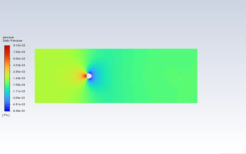
Pressure
Reynolds no-100
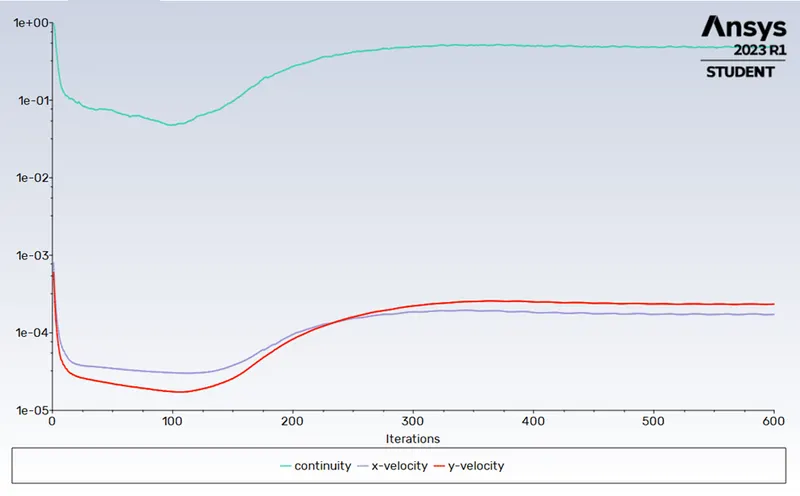
Residual plots
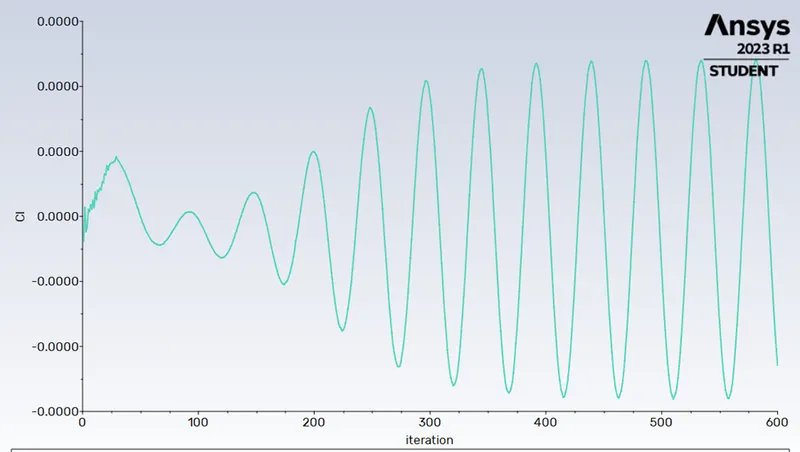
Coefficient of lift
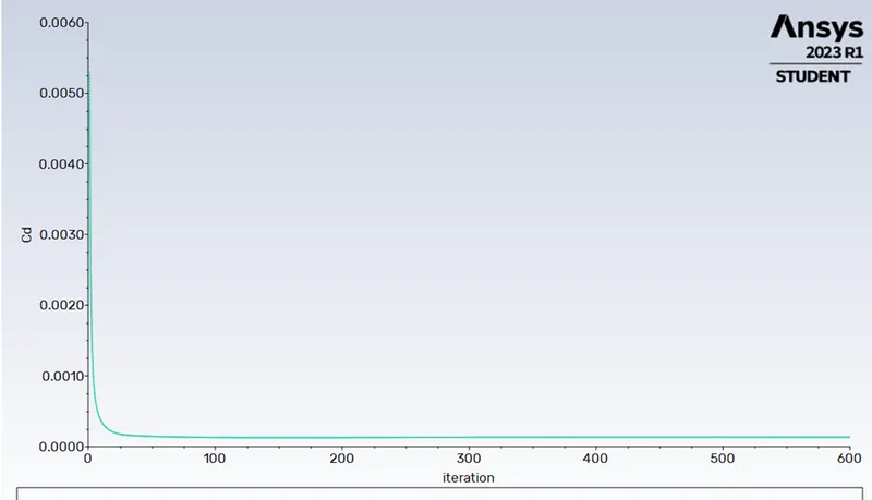
Coefficient of drag
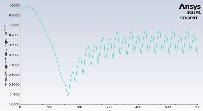
Vertex velocity at monitor point
Contours plots-
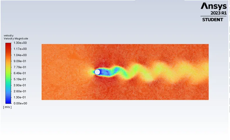
Velocity
Pressure
Reynolds no-1000
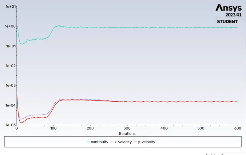
Residual plots
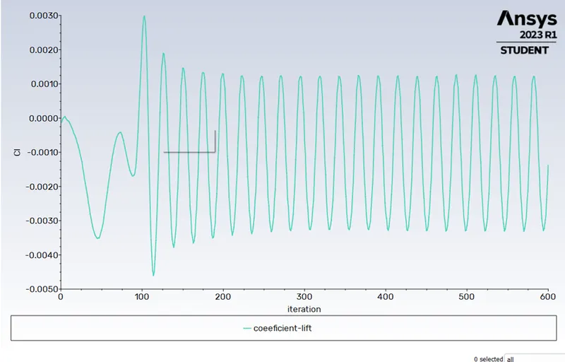
Coefficient of lift
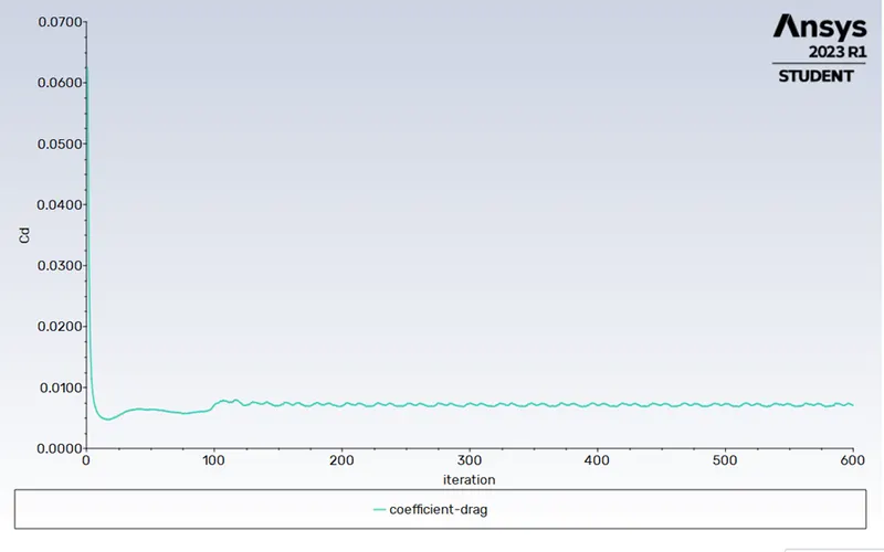
Coefficient of drag
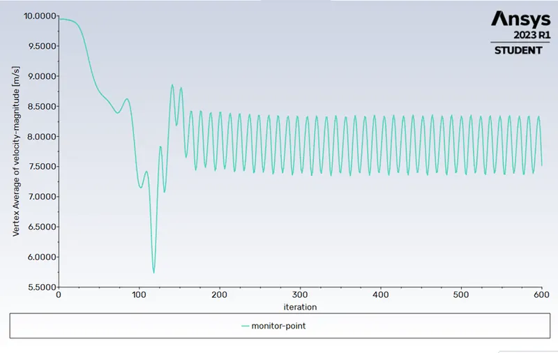
Vertex velocity at monitor point
Contours plots-
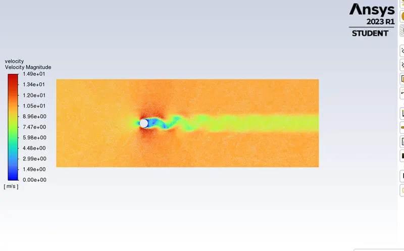
Velocity
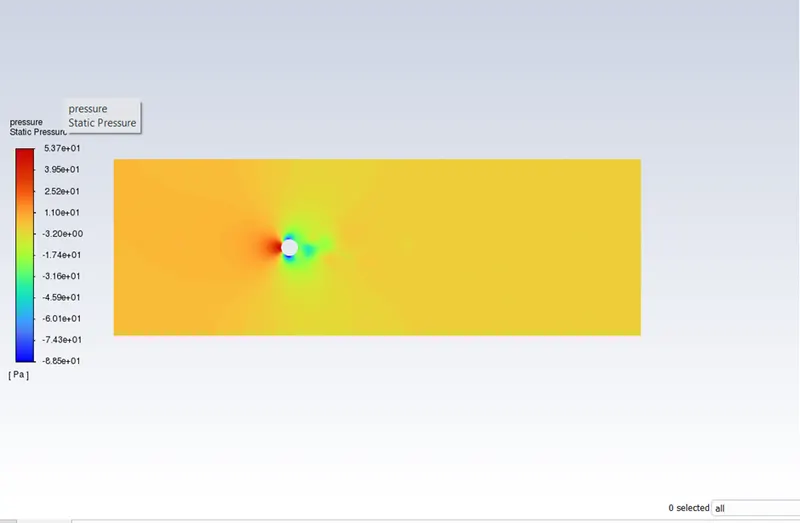
Pressure
Reynolds no-1000
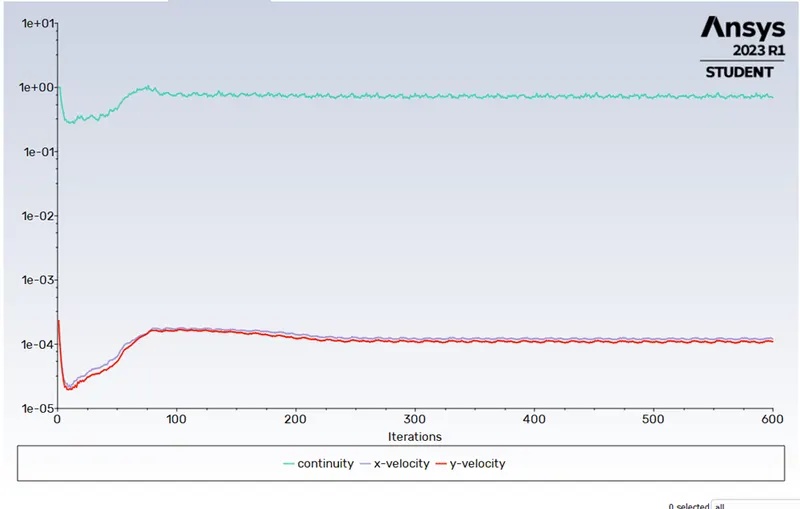
Residual plots
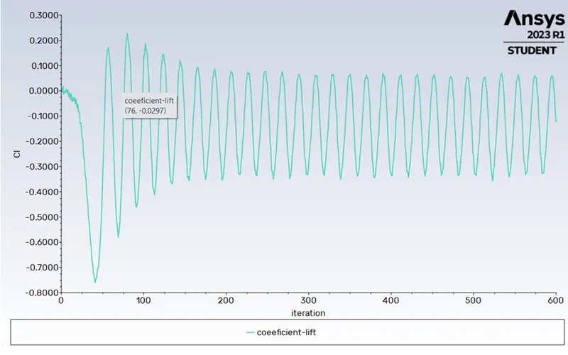
Coefficient of lift
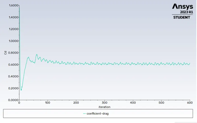
Coefficient of drag
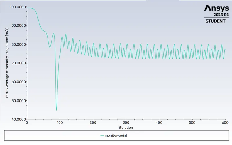
Vertex average
Contour plots –
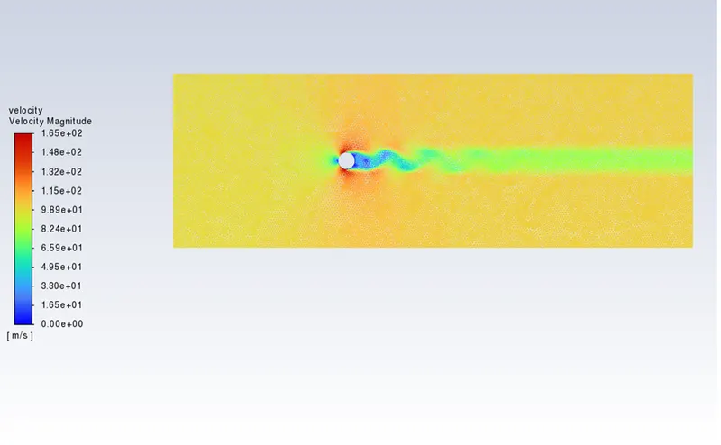
Velocity
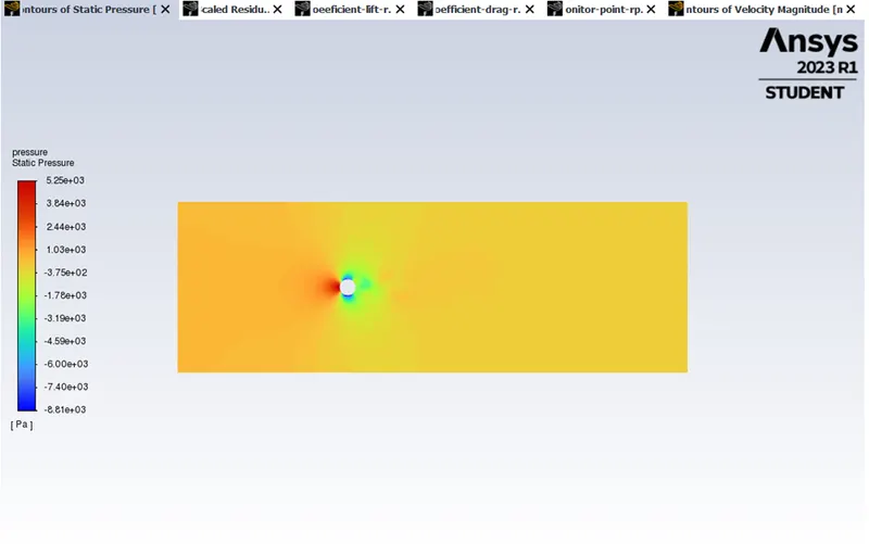
Pressure
Reynolds no-10000
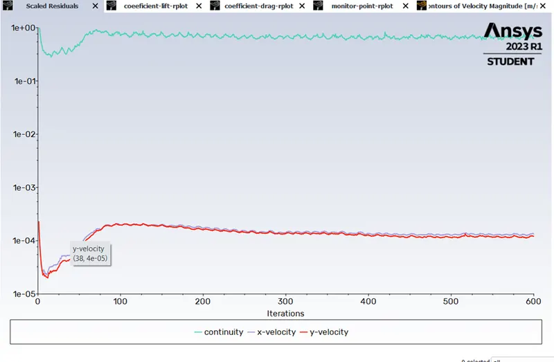
Residual plots
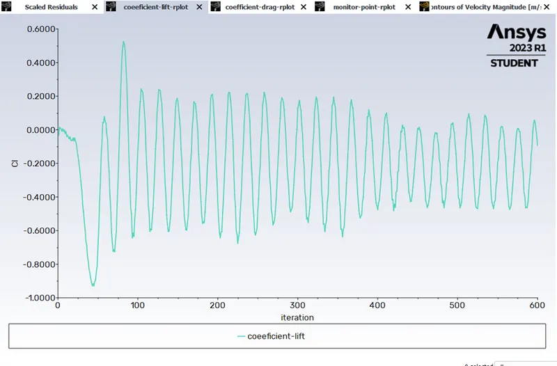
Coefficient of lift
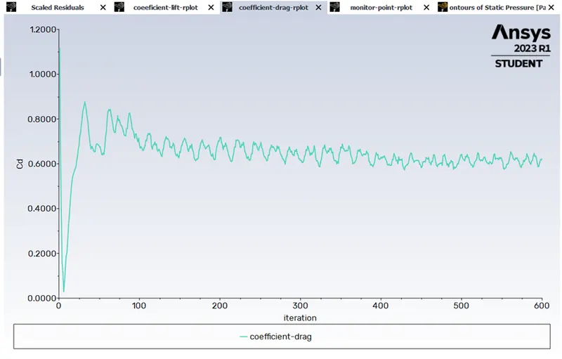
Coefficient of drag
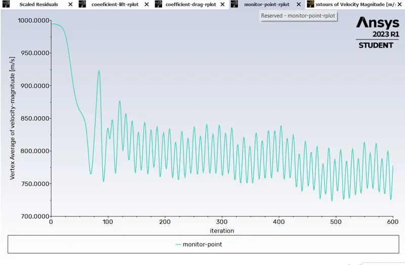 Vertex average
Contour plots –
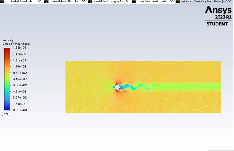
Velocity
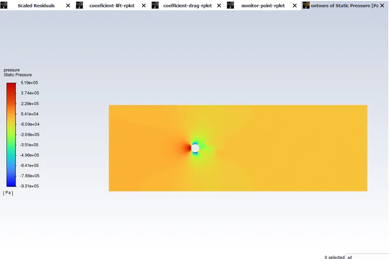
Pressure
Below are the dimensionless variable
Coefficient of drag - CD=2Fd/ ρ V2A
Coefficient of lift - CL=2L/ ρ V2A
|
Reynolds no |
velocity |
cd |
cl |
Vertex velocity |
|
10 |
0.1 |
3.32e-06 |
4.04e-09 |
-0.05 |
|
100 |
1 |
0.0013 |
-1.143e-03 |
0.518 |
|
1000 |
10 |
0.007 |
-0.00135 |
7.5 |
|
10000 |
100 |
0.627 |
-0.1267 |
77.26 |
|
100000 |
1000 |
0.624 |
-0.094 |
777.3996 |
Conclusions : After inspecting the plots and contours provided above, with the increase in Reynold number the drag-coefficient slightly decreases and the lift-coefficient increases.