Simulating cyclone separator with DPM

Aim : To perform analysis on cyclone separator and calculate the separation efficiency and pressure drop.

Objectives :

1. To write a few words about any four empirical models used to calculate the cyclone separator efficiency. 
2. To perform an analysis on a given cyclone separator model by varying the particle diameter from 1 μm to 5 μm and calculate the separation efficiency in each case. Discuss the results. [Use both the velocity's as 3m/sec.]
3. To perform an analysis on a given cyclone separator model by varying the particle velocity from 1 m/sec to 5 m/sec and calculate the separation efficiency and pressure drop in each case. Discuss the results. [Use particle diameter size as 5 μm for all cases & keep flow velocity same as particle velocity]

4. Boundary Conditions:-
   1. Inlet and wall:- Reflect
   2. Outlet(Top):- Escape 
   3. Outlet(Bottom/dustbin) – Trap
5. Structural mesh gives the best results, so you can use cutcell meshing approach available in Ansys Meshing.

Theory :

1.     Cyclone separator :

• Cyclone separators are the separation devices which separate the particulate matter from the flue gas.
• The cyclone separator is a common separation and classification equipment, which uses the principle of centrifugal sedimentation.
• When the mixed liquid to be separated enters the cyclone tangentially from the periphery of the cyclone at a certain pressure, strong 3-dimensional elliptical strong rotating shear turbulence is generated.
• They used the principle of inertia to separate the particles from the flue gas.
• Cyclone separators are used in many industries due to their low cost, simple in design and high efficiency.

2.     Cyclone separator efficiency :

• The cyclone separation efficiency is given by the ratio of the total number of particles trapped to the total number of particles tracked.

`ɳ= ("no.of particles trapped")/("no.of particles tracked")`

• As particle size increases, the efficiency also increase.
• As particle velocity increase, the efficiency also increase.
• There are 4 empirical model are used to calculate the cyclone separator efficiency as follows
  1. Iozia and Leith Model
  2. Lapple Model
  3. Koch and Licht Model
  4. Li and Wang Model

Lets see one by one

2.1.           Iozia and Leith model :

• Iozia and Leith logistic model is a modified version of Barth Model, which is developed based on force balance.
• The model assumes that a particle carried by the vortex endures the influence of two forces: a centrifugal force and a flow resistance. The collection efficiency ɳ_i of particle diameter (d_pi) can be calculated as

`ɳ_i= 1/(1+ (d_(pc)/d_"pi")^β )`

Where β is an expression for slope parameter derived based on the statistical analysis of experimental data of a cyclone with D=0.25m

`β=0.62-0.87 ln⁡(d_"pc"/100)+5.21ln⁡((ab)/D^2 )+1.05[ ln⁡((ab)/D^2 ) ]^2`

And d_pc is the 50%cut size given by Barth

`d_"pc"=[(9μQ)/(πρ_p z_c v_(t max)^2 )]^0.5`

Where z_c = core length

2.2.           Lapple model :

• Lapple model was developed based on force balance without considering the flow resistance.
• Lapple assumed that a particle entering the cyclone is evenly distributed across the inlet opening. The particle that travels from inlet half width to the wall in the cyclone is collected with 50% efficiency. The semi empirical relationship developed by Lapple to calculate a 50% cut diameter, dpc, is

`d_"pc"=[(9μb)/(2πN_e v_i (ρ_p-ρ_g))]^0.5`

Where N_e is the number of revolutions

The efficiency of collection of any size of particle is given as,

`ɳ_i= 1/(1+ ((d_"pc")/bar(d_"pi"))^2`

2.3.           Koch and Licht model :

• Koch and Licht collection theory recognized the inherently turbulent nature of cyclones and the distribution of gas residence times within the cyclone.
• Koch and Licht described particle motion in the entry and collection regions with the additional following assumptions:
  • The tangential velocity of a particle is equal to the tangential velocity of the gas flow, i.e. there is no slip in the tangential direction between the particle and the gas.
  • The tangential velocity is related to the radius of cyclone as `uR^n="constant".`
• The force balance and an equation on the particles collection yields the grade efficiency ηi

`ɳ_i=1-exp⁡{-2[(Gtau_i Q)/D^3 (n+1) ]^(0.5/(n+1)) }`

Where,

 `G= (8K_c)/(K_a^2 K_b^2 )`

 `n=1-{1- (12D)^0.14/2.5}{(T+460)/530}^0.3`

`tau_i= (ρ_p d_"pi"^2)/(18μ)`

Where, G is a factor related to the configuration of the cyclone, n is related to the vortex and τ is the relaxation term.

2.4.           Li and Wang model :

• The Li and Wang model includes particle bounce or re-entrainment and turbulent diffusion at the cyclone wall. A two dimensional analytical expression of particle distribution in the cyclone is obtained.
• Li and Wang model was developed based on the following assumptions:
  • The radial particle velocity and the radial concentration profile are not constant for uncollected particles within the cyclone.
  • Boundary conditions with the consideration of turbulent diffusion coefficient and particle bounce re-entrainment on the cyclone wall are: 

    c = c₀,  at θ = 0

    `D_r (∂c)/(∂r)=(1-α)ωc`, at r=D/2

  • The tangential velocity is related to the radius of cyclone as, `uR^n="constant"`.

• The resultant expression of the collection efficiency for particle of any size is given as,

`ɳ_i=1-exp⁡(-λθ_1)`

Where,

 `λ=((1-α)Kw_w)/(D_r r_w^n )`

`theta_1` = 2π(S + L)/a

3.     Discrete phase model(DPM) :

• The lagrangian discrete phase model in ansys fluent follows the Euler-Lagrange approach.
• The fluid phase is treated as continuum by solving the Navier-Stokes equations, while the dispersed phase is solved by tracking a large number of particles, bubbles or droplets through the calculated flow field.
• The dispersed phase can exchange momentum, mass and energy with the fluid phase.
• A fundamental assumption made in this model is that the dispersed second phase occupies a low volume fraction(<10%).
• The particle or droplet trajectories are computed individually at specified intervals during the fluid phase calculations.
• Massles, inert, droplet, combusting and multicomponent type of particles used as a injections in the DPM.
• The applications of DPM in industries as IC engine fuel injection system, spray modelling, vacuum cleaner analysis etc.
• There are following boundary conditions are used in this model
  1. Reflect : the particle rebounds off the boundary in question with change in its momentum as defined by the coe. of restitution.
  2. Trap : the trajectory calculations are terminated and the fate of the particle is recorded as trapped.
  3. Escape : the particle is reported as having escaped when it encounters the boundary in question. Trajectory calculations are terminated.
  4. Wall-jet : the direction and the velocity of the droplet particles are given by the resulting momentum flux, which is function of the impingement angle (`φ`) and the weber number(Wb). The wall-jet boundary condition is appropriate for high temp walls where no significant liquid film is formed and high Wb impacts where the spray acts as a jet.
  5. Wall film : this B.C. consist of four regimes as stick, rebound, spread and splash which are based on the impact energy and wall temp.

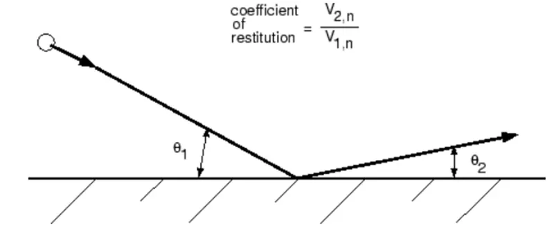
Fig : reflection of particle

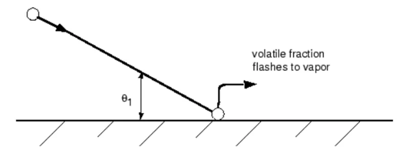
Fig : trap of molecule

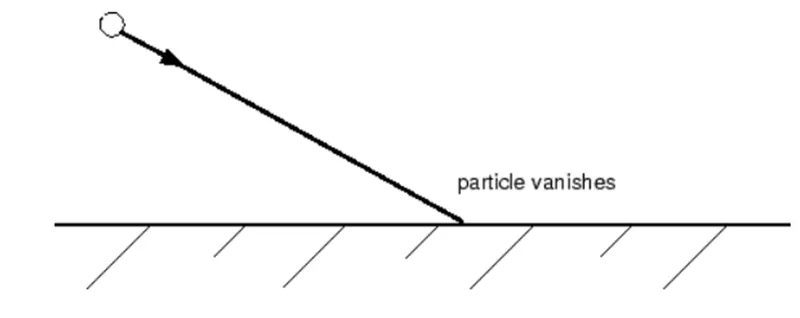
Fig : escape of particle

Modelling approach :

1.     Pre-processing methods :

1.1.           Geometry :

• Open ansys workbench
• Drag fluid flow (fluent) to project scheme.
• Open spaceclaim

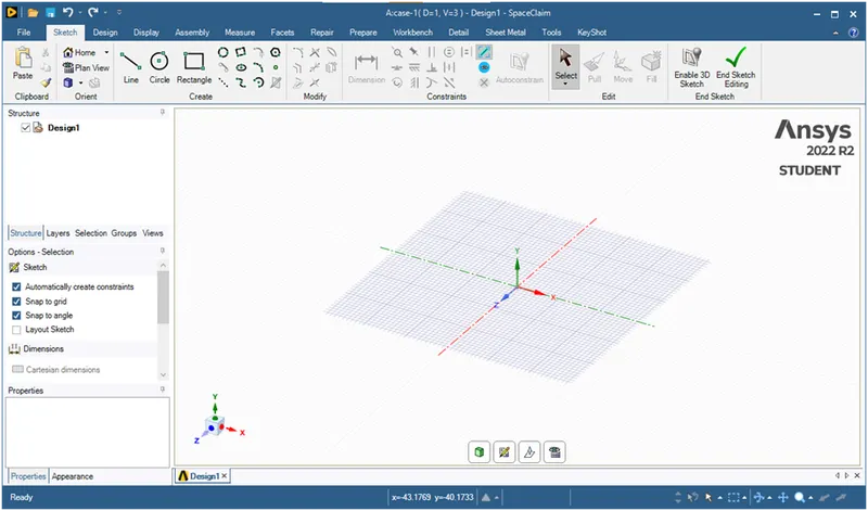
• Import the geometry file

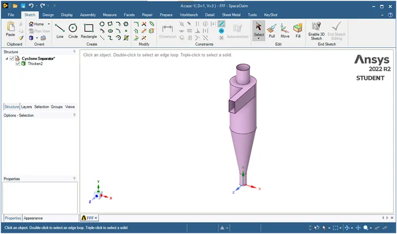
• Extract the fluid volume

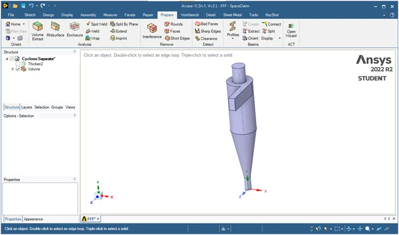
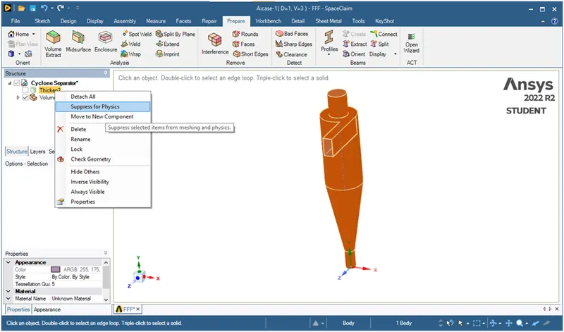
• Suppress the solid part or sheet metal for physics

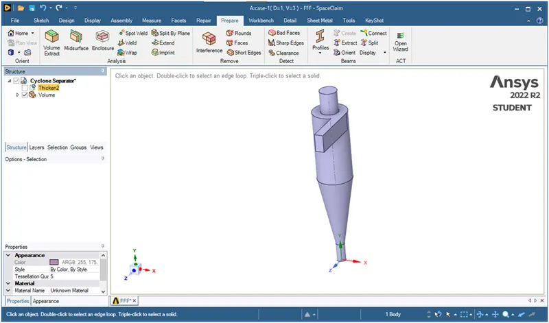
Then close the space-claim and open mesh.

1.2.           Meshing :

• Open mesh

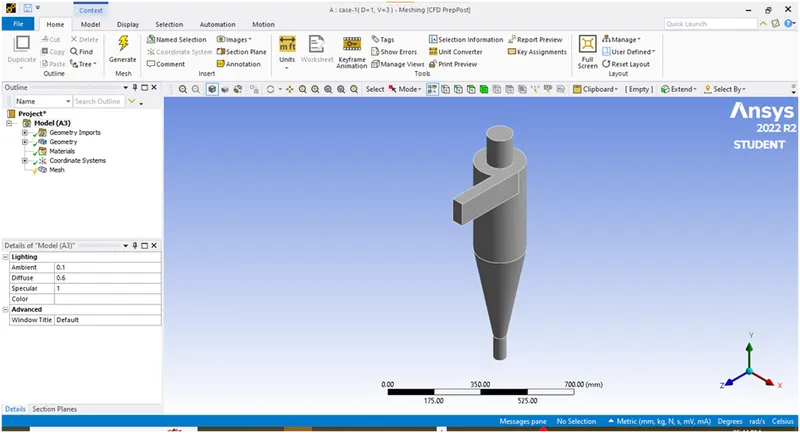
• Right click on mesh and generate mesh

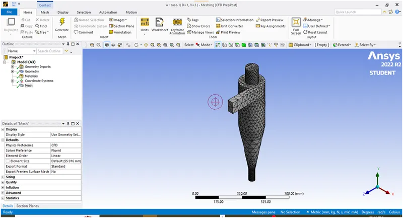
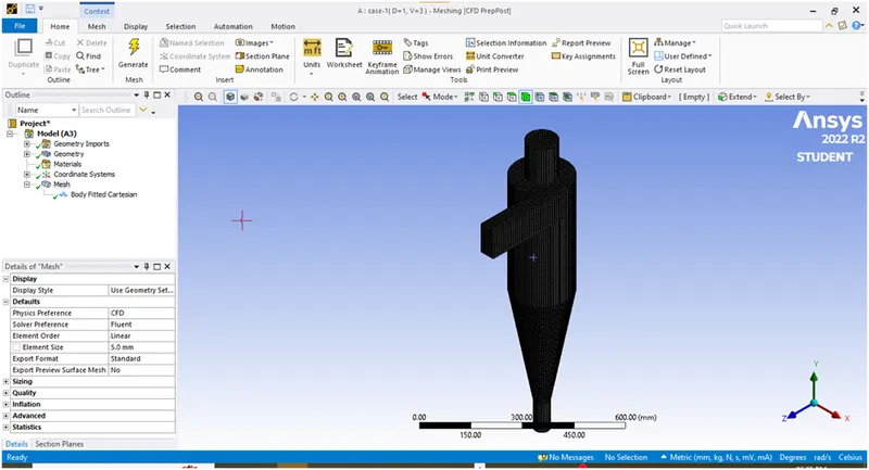
This is a course mesh and here the triangle i.e. unstructured mesh created. But as per given problem statement we have to use cutcell method for that delete this mesh and add meshing method as Cartesian mesh with size 5mm to track more number of particals.

• Lets gives the names to the selected faces as shown below

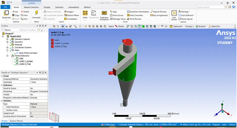
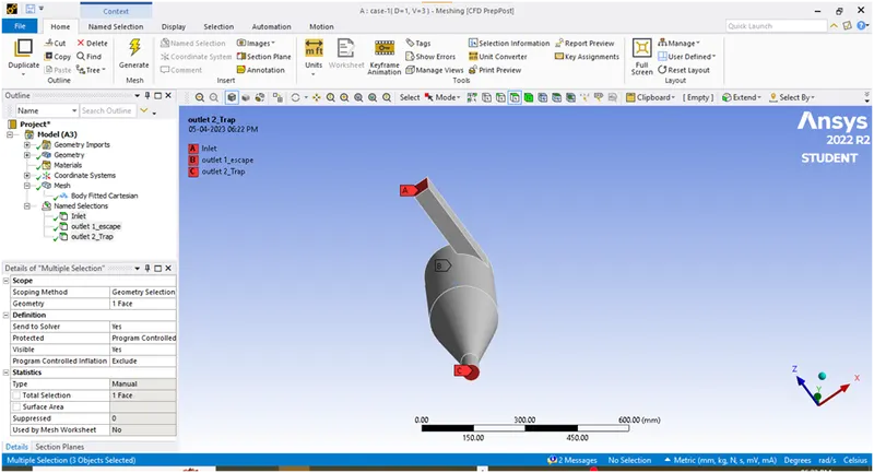
Now it’s done. Just click on update to transfer the data to fluent. close the mesh.

2.     Post-processing methods :

2.1.           Setup:

• Open ansys fluent by right clicking on setup

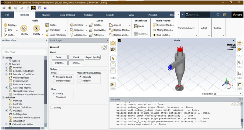
• Enabled gravity in y-direction as -9.81m/s2
• We are using pressure based solver and steady state time analysis
• Now goto models

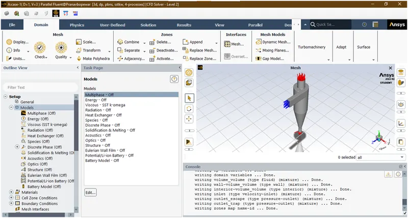
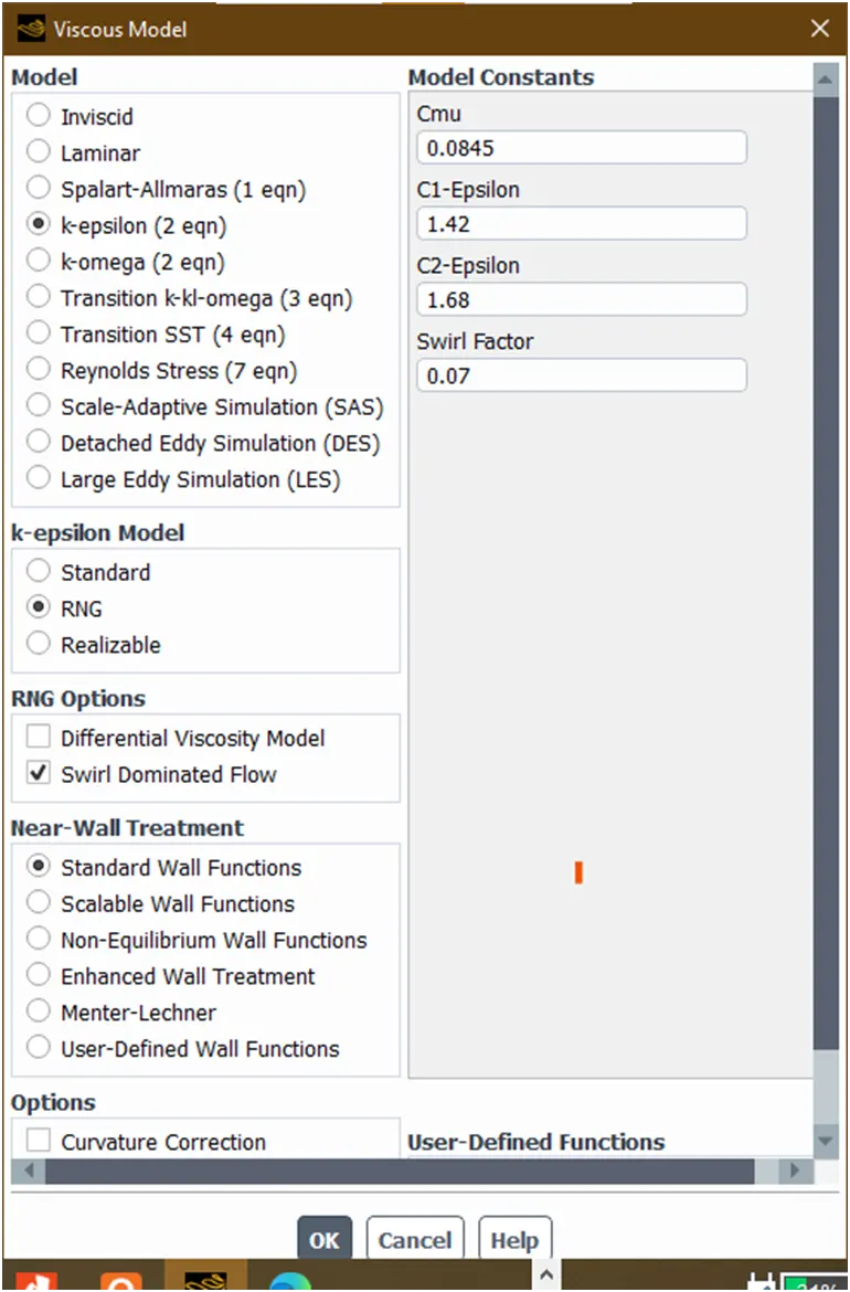
Now enabled viscous-k-epsilon-RNG-swirl model

Now goto discrete phase model

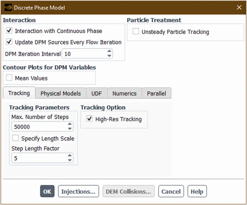
Then goto injections and add surface type injection and select particle as anthracite at inlet surface with diameter=1 µm and particle velocity= 3m/s as shown below

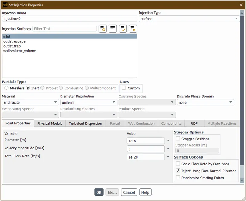
Now click on ok..

• Now goto boundary conditions and apply as shown below

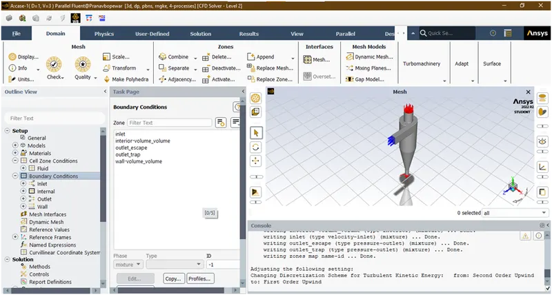
Goto inlet and select velocity=3m/s, in dpm select boundary type as reflect because we don’t want to escape the particles from inlet.

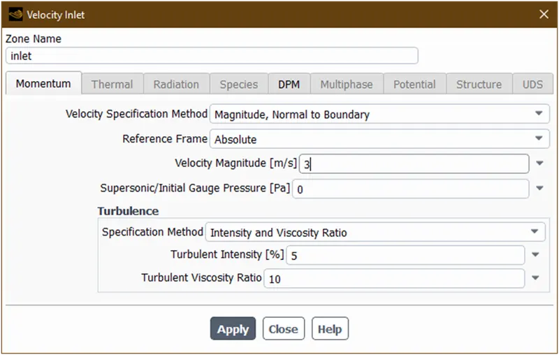
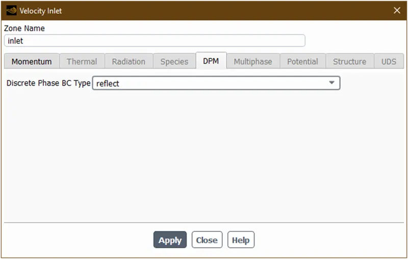
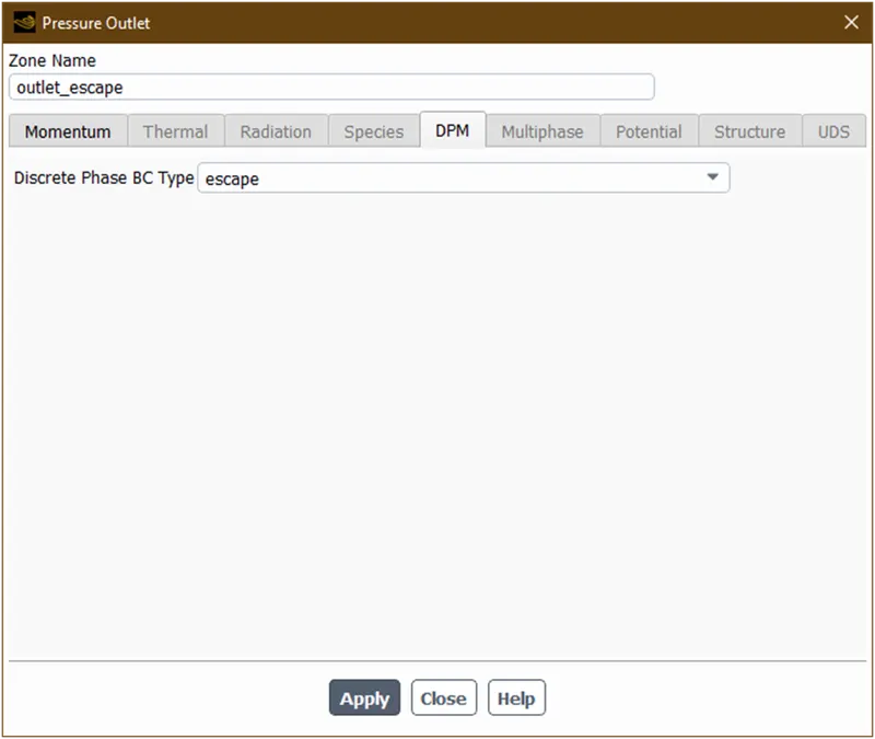
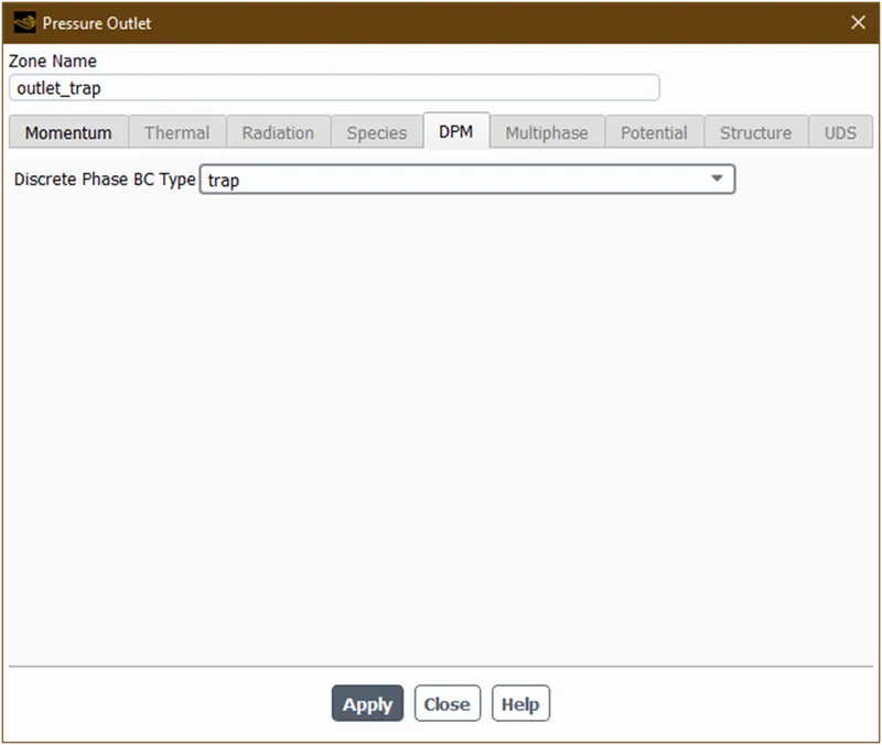
Now click on apply . its done

• Lets goto solution-> methods

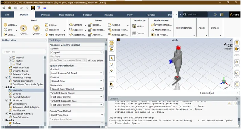
Select coupled method because in this it gives best results and change from first order upwind to 2^nd order upwind because it reduces computational time and also provides best solution compared to 1^st order upwind.

• Goto initialization and select standard initialization method because this model has multiple no. of inlets and outlets.
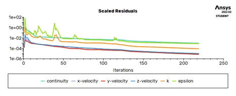
• Now click on run calculation under solution and run this solution for almost 500 iterations. Till the solution is converged.

2.2.           Plotting results :

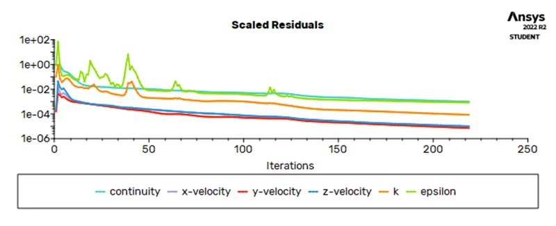
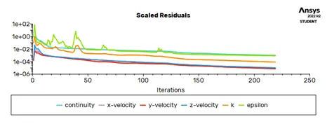
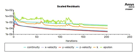
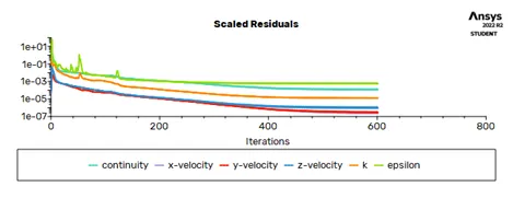
• Residual plot

• Particle track

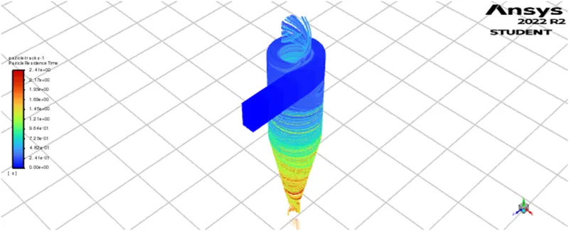
From this the separation efficiency can be calculated as

`ɳ= ("no.of particles trapped")/("no.of particles tracked")`

`ɳ= 299/378xx100=79.10%`

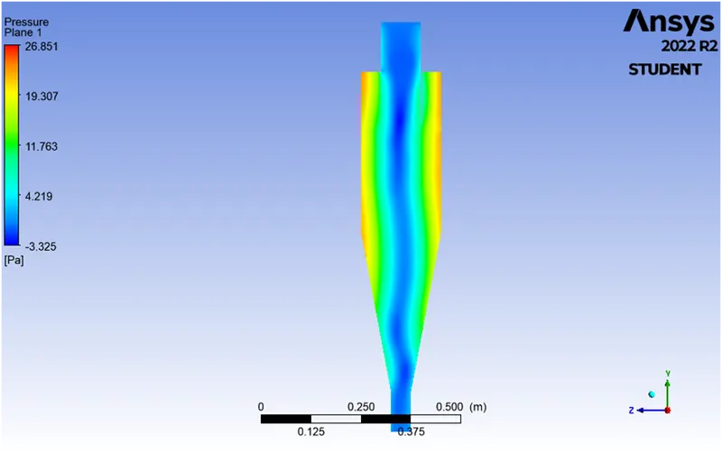
• Lets calculate pressures at inlet and outlet and calculate pressure drop

Inlet pressure(Pi) = 31.34 Pa

Total outlet pressure(Po) = 4.30 Pa

Pressure drop = Pi – Po = 27.04 Pa

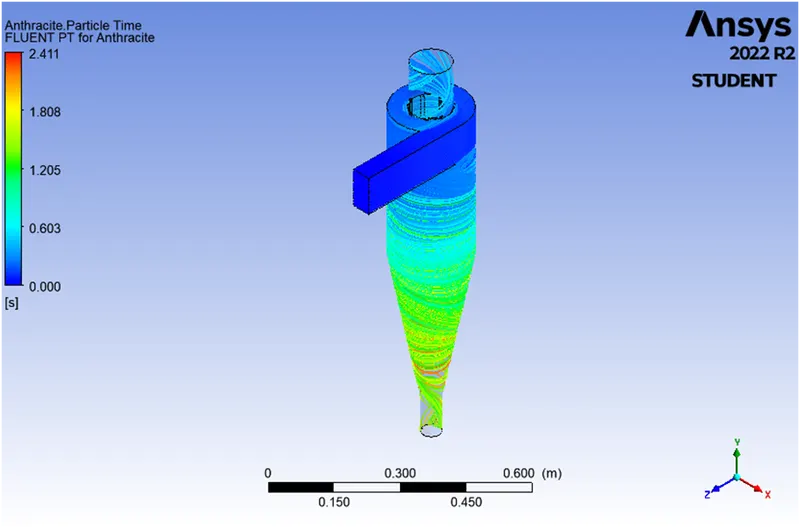
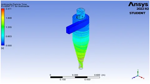
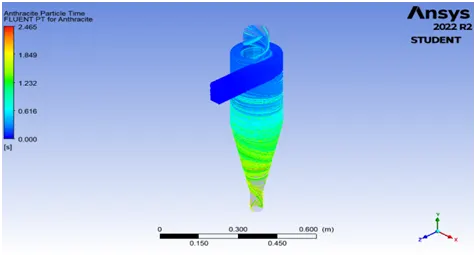
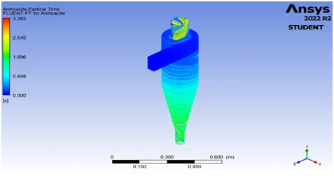
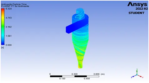
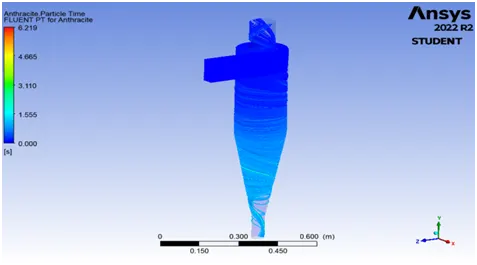
• Firstly export the particle data history to cfd post and then import the particle history data time in cfd post. Then plot the graph

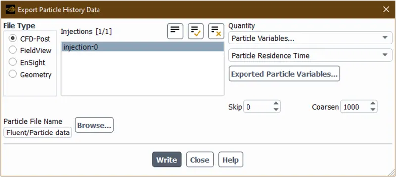
Now open cfd post and then import the file

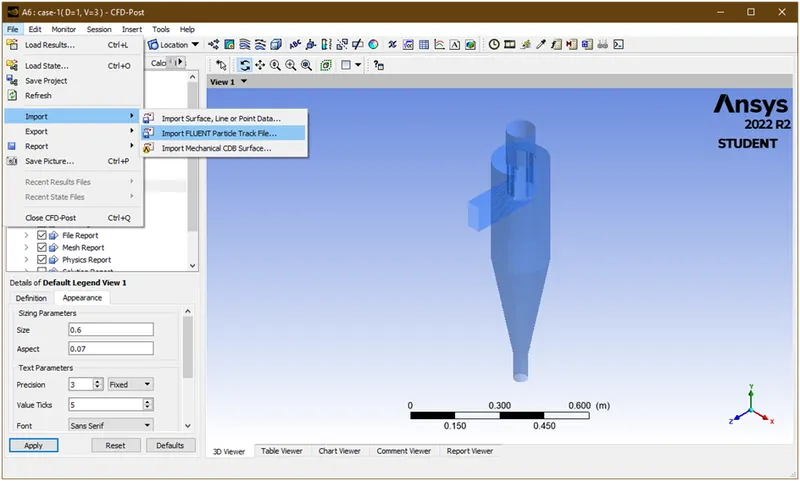
Now plot the particle time

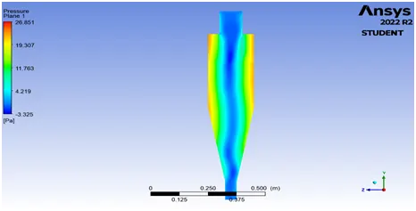
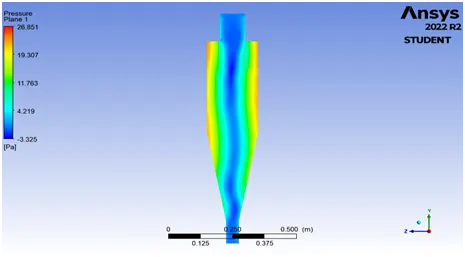
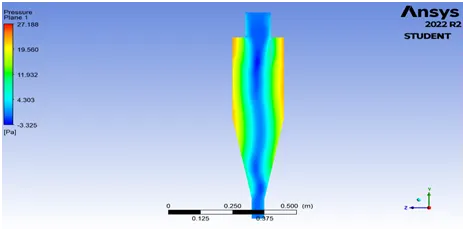
• Lets plot velocity and pressure contour plots on a plane

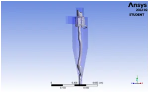
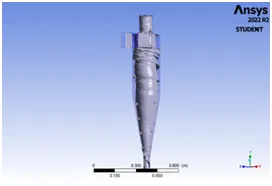
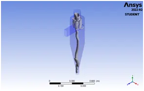
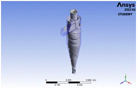
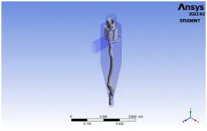
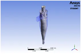
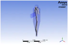
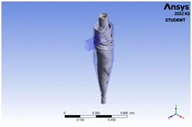
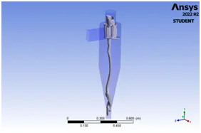
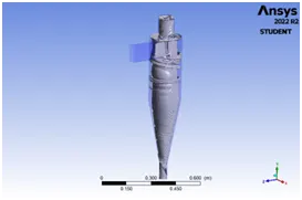
• Lets plot vortex core region

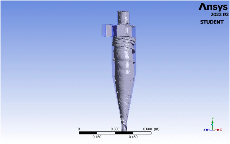
• Now for more cases just repeat the procedure by just changing the input data which is provides in problem by varying first particle size and then by varying particle velocity.

Results :

• Finding out separation efficiency and pressure drop

Case no.	Particle size(µm)	Particle velocity (m/s)	No. of particles tracked	No. of particles trapped	Separation efficiency	Inlet pressure ( pa)	Outlet pressure(Pa)	Pressure drop (Pa)
1	1	3	378	299	79.10	31.34	4.30	27.04
2	3	3	378	306	80.95	31.34	4.30	27.04
3	5	3	378	308	81.48	31.35	4.30	27.05
4	5	1	378	310	82.01	2.871	0.378	2.493
5	5	5	378	274	72.48	91.84	12.72	79.12

• Residual plots

Case no.	Particle size(µm)	Particle velocity (m/s)	Residual plots
1	1	3
2	3	3
3	5	3
4	5	1
5	5	5

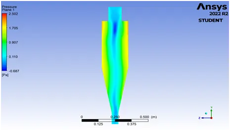
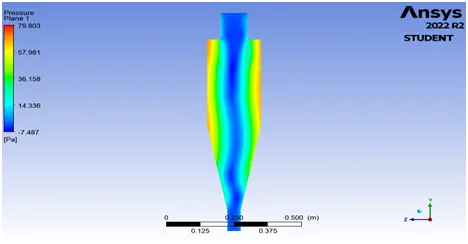
• Pressure contours

Case no.	Particle size(µm)	Particle velocity (m/s)	Pressure contours
1	1	3
2	3	3
3	5	3
4	5	1
5	5	5

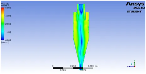
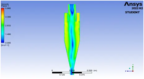
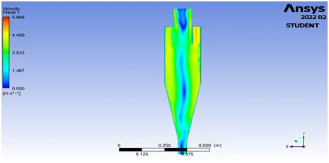
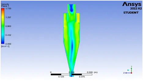
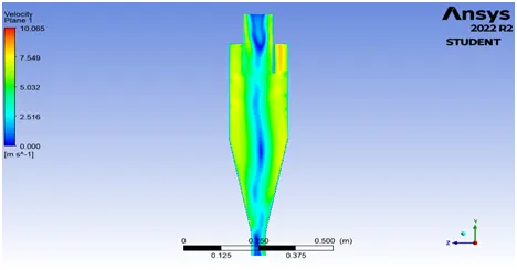
• Velocity contours

Case no.	Particle size(µm)	Particle velocity (m/s)	Velocity contours
1	1	3
2	3	3
3	5	3
4	5	1
5	5	5

• Vortex core region

Case no.	Particle size(µm)	Particle velocity (m/s)	At centre	Near wall
1	1	3
2	3	3
3	5	3
4	5	1
5	5	5

• Particle track time plot

Case no.	Particle size(µm)	Particle velocity (m/s)	Particle track plots
1	1	3
2	3	3
3	5	3
4	5	1
5	5	5

Conclusions :

• From the table I can conclude that as particle size increases the cyclone separation efficiency also increases.
• From table I can conclude that as particle velocity increases the cyclone separation efficiency gets decreased.
• From table I can conclude that, as particle velocity increases the pressure drop also increased.
• From residual plots I can say that the solution gets converged at 210 iterations.
• From pressure contours I can say that, as particle size increases, the pressure at wall also increased and at core the low pressure is developed due to centrifugal force.
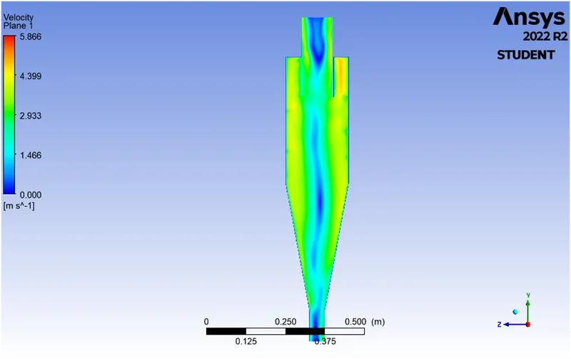
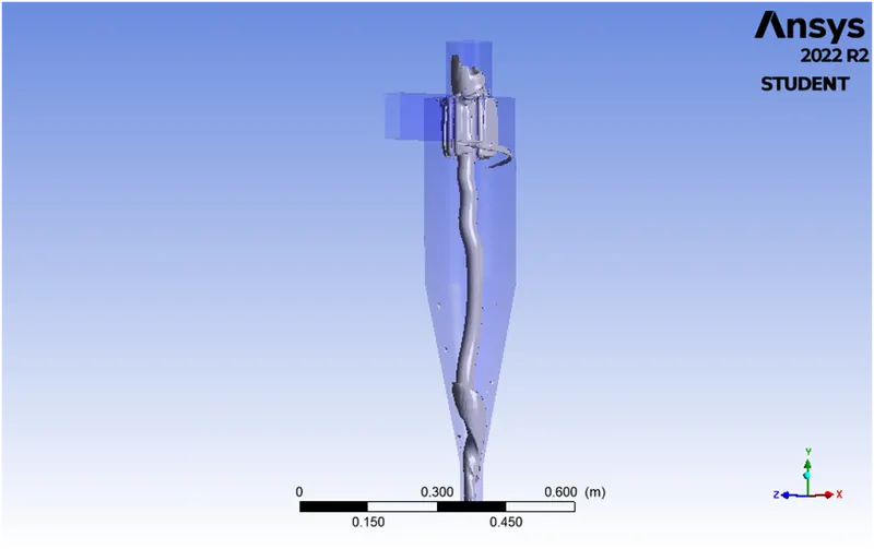
• From velocity contours I can say that, the velocity at centre is very low due to centrifugal force dominates over the drag force.
• From particle track time plots, I can say that as the particle size increases the particle are takes more time to escape and also for trap. And also as velocity increases the particle track time gets reduced.