Week 8 - Simulating Cyclone separator with Discrete Phase Modelling

AIM:-

To Run the Simulation on a Cyclone Separator and to calculate the Seprartion Efficiency and Pressure drop Using Ansys-Fluent.

OBJECTIVE:-

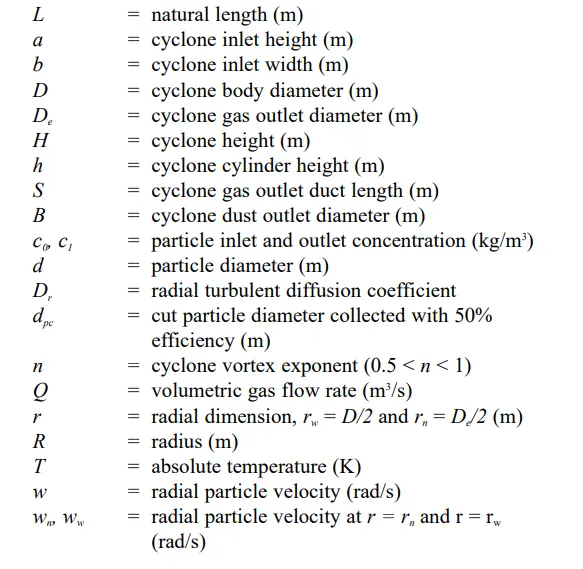
1. To write a few words about any four empirical models used to calculate the cyclone separator efficiency.
2. To perform an analysis on a given cyclone separator model by varying the particle diameter from 1 μm to 5 μm and calculate the separation efficiency in each case. Discuss the results. [Use both the velocity's as 3m/sec.]
3. To perform an analysis on a given cyclone separator model by varying the particle velocity from 1 m/sec to 5 m/sec and calculate the separation efficiency and pressure drop in each case. Discuss the results. [Use particle diameter size as 5 μm for all cases & keep flow velocity same as particle velocity]

BOUNDARY CONDITIONS :-

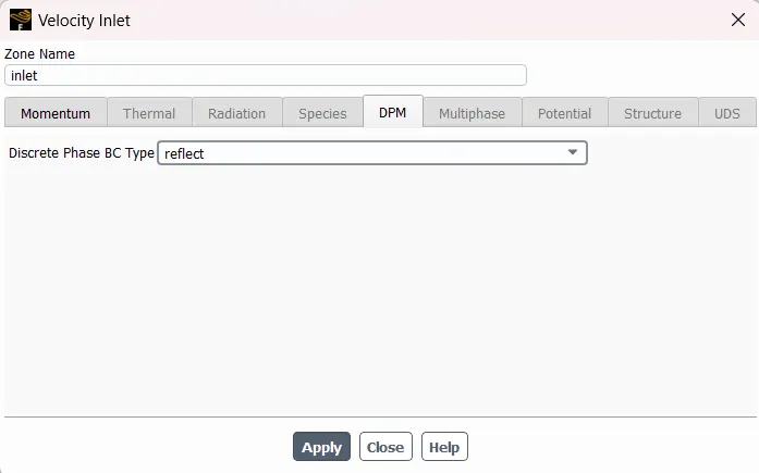
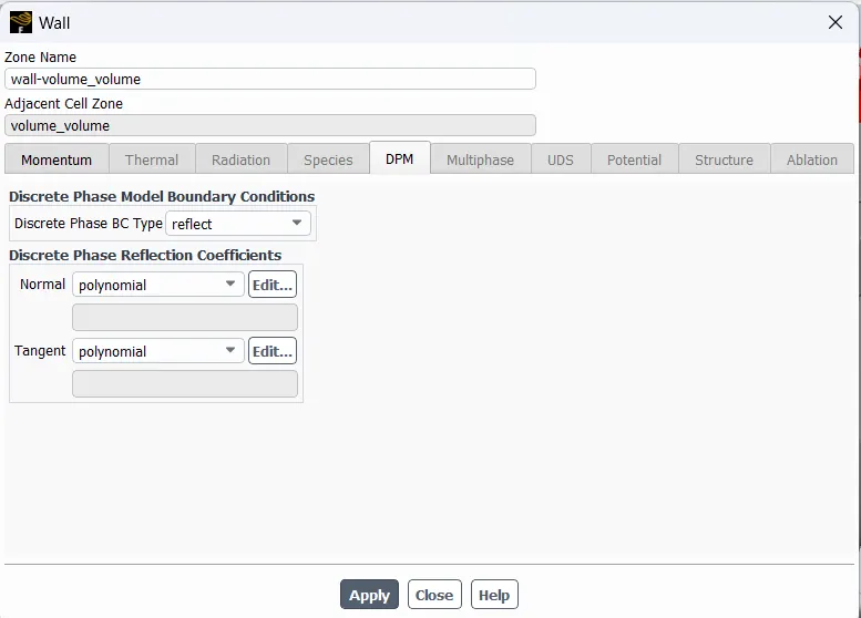
Inlet and wall:- Reflect

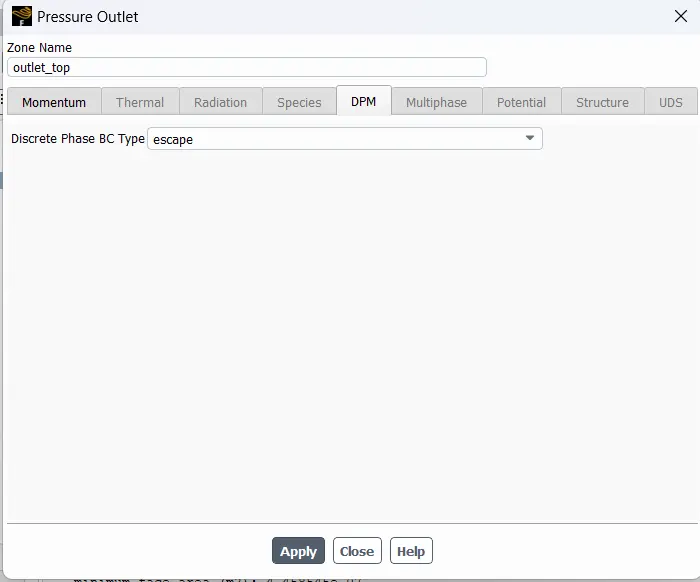
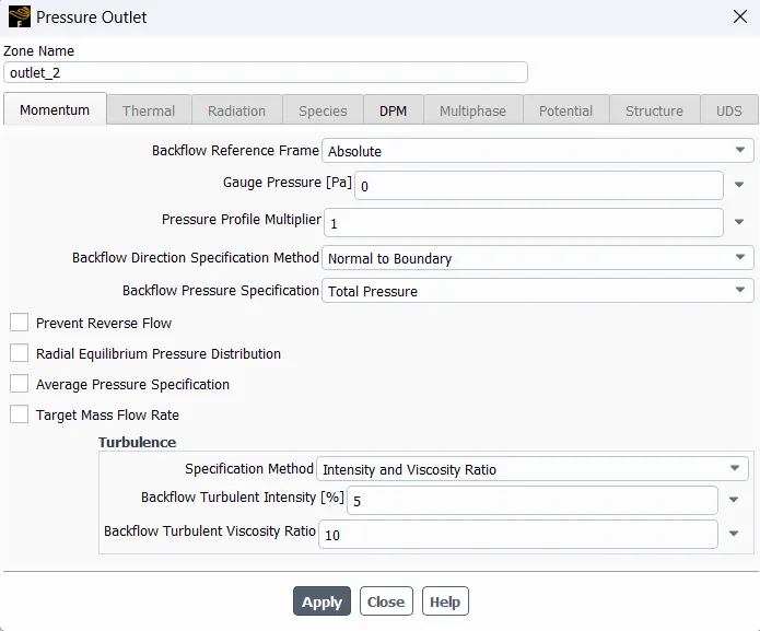
Outlet(Top):- Escape

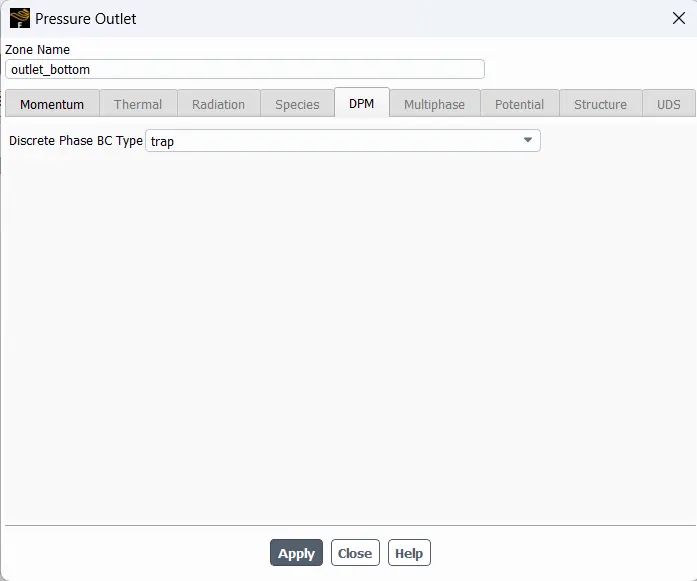
Outlet(Bottom/dustbin) - Trap

PROCEDURE:-

CYCLONE SEPARATOR

Cyclone Separators or simply Cyclones are Separation Devices (Dry Scrubbers) that uses the principle of Interia to remove particulate matter from flue gases. Cyclone Separators is one of many air population control devices known as Preclearners. Since they generally remove larger pieces of particulate matter. This Prevents finer filtration methods from having to deal with large, more abrasive particle later on. In addition, Cyclone Separator can Operate in parallel, and this system is known as Multicyclone.

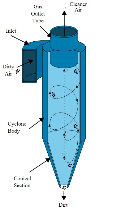
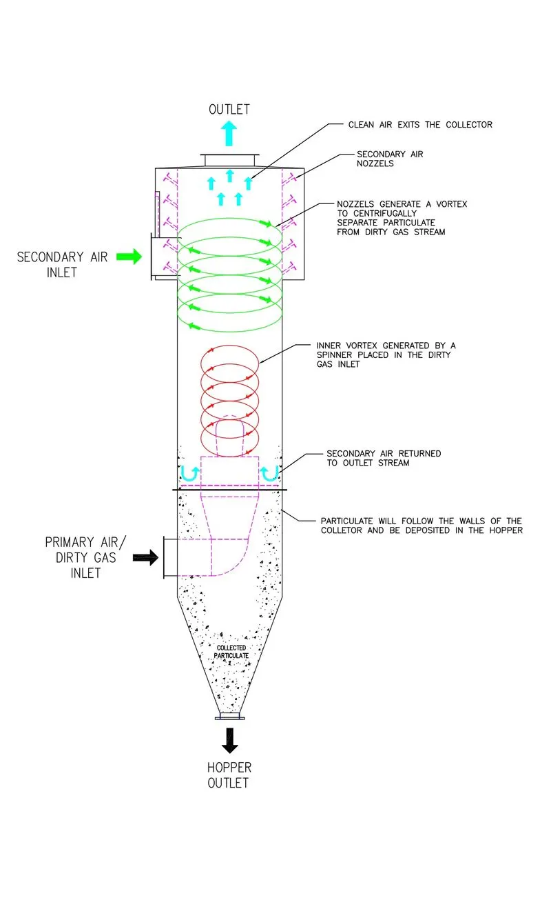
It is important to note that Cyclone can vary drastically in their Size. The Size of Cyclone depends largely on how much flue gas must be fittered, thuslarger Operations tend to need larger cyclones. For example, Several different models of one cyclone type can exist and Size can range form a relatively small 1.2 to 1.5m tall (about 4 to 5 feet) to around 9 meters (30 feet) which is about tall as a three story building.

• WORKING PRINCIPLE.

Cyclone Separators work much like a centrifuge, but with a continous feed of dirty air. In Cyclone Separator, dirty flue gas is fed into a chamber create a spiral vortex similar to a torando. This Spiral formation and sepration is known as Strom. The lighter components of gases have less interia. So it is easier for them to be influenced by vortex and travel up it. Contrasily, larger Components of particular matter have, more interia and are not as easily influenced by vortex.

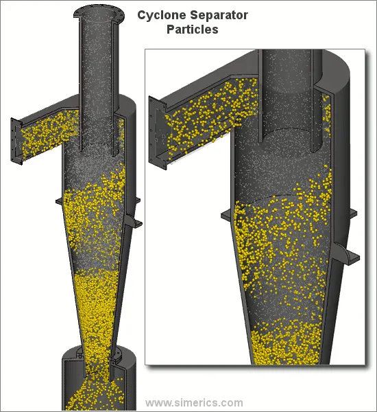
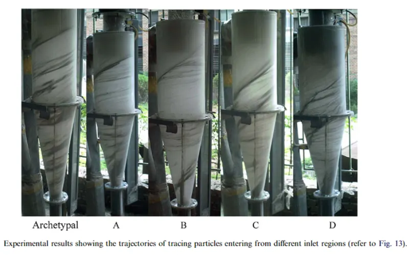
Since these larger particles have difficulty following the high-speed spiral motion of gas and the vortex, the particle hit inside walls of the container and drop down into a collection hopper. These Chambers are Shaped like a Upside-Down Cone to promote the collection of these particles at the bottom of the container. The cleaned flue gases escapes out of the Chamber.

Most Cyclones are built to control and remove particulate matter that is larger than 10 mirometers in diameter. However, there do exist high efficiency cyclones that are designed to effective on particles as small as 2.5 micrometers. As well, these Separators are not effective on extermely large particulate matter. For particulate around 200 micrometers in size, gravity setting Chambers or Momentum Separators are the better options.

Out of all of particulate-control devices, cyclone separators are among the least expensive. They are often used as a pre-treatment before the flue gas enters more effective pollution control devices. Therefore Cyclone Separators can be seen as Rough Separators before the flue gas reaches the fine Filtration Stages.

ADVANTAGES.

• Cyclone Separators are benificals because they are not expensive to install or maintain and they have no moving parts.
• This keeps the maintenance and operating cost low.
• The removed particulate matter is collected when dry, which makes it easier to dispose of.

DIS-ADVANTAGES.

• Standard models are not able to collect particulate matter that is smaller than 10 micrometer, effectively and the machines are unable to handle Sticky or Tacky materials well.

• DERIVATION - (WIKIPEDIA)

As the Cyclone is essentially a two-phase particle-fluid system, Fluid Mechanics and Particle transport equations are used to describe the behaviour of cyclone. The air in a Cyclone is initially introduced tangentially into a cyclone with an inlet Velocity V_in. Assuming that particle is Spherial, a Simple analysis to calculate critical separation particle Size can be established.

If One considers an isolated partcile circilng in the upper cylinderical component of the cyclone at a rotational radius `r` from the cyclone's central axis the particle is therefore subjected to Drag, Centrifugal, Buoyant Forces. Given that the fluid velocity is moving in a spiral, the gas velocity can be broken into two component velocities a tangential component, `V_t` and outward radial velocity component `V_r`. Assuming Stoke's Law the Drag Force in the outward radial direction that is opposing the outward radial direction that is opposing the Outward Velocity on any particle in inlet stream is

`F_d rarr -6*pi*r_p *mu*V_r`

Using`rho_p` as particle's density, the centrifugal component Outward radial is

`F_c rarr (m *V_t^2)/r rarr 4/3 pi*rho_p*r_p^3*V_t^2/r`

The buoyant force component in the inward radial direction. It is in the Opposite direction to the particle's centrifugal force because it is on a Volume of Fluid that is missing compared to the Surrounding Fluid. Using for the density of the fluid, the buoyant force is

`F_b rarr - V_p *rho_f*V_t^2/r rarr-4/3pi*r_p^3*V_t^2/r*rho_f`

In this case, is equal to volume of particle(as opposed to velocity). Determing the Outward Radial Motion Of Each Particle is found by setting NEWTON's SECOND LAW OF MOTION equal to Sum of these FORCES.

`m*(dV_r)/dt rarr F_d +F_c+F_b`

We can assume the particle under consideration has reached Terminal Velocity. that is acceleration `(dV_r)/dt` is zero.

This Occur when the radial velocity has caused enough Drag Force to contour the Centrifugal and Buoyancy Force. This Simplification changes equation to

`F_d +F_c+F_b rarr 0`

`-6pir_p mu V_r +4/3pi r_p^3V_t^2/r rho_p-4/3pir_p^3V_t^2/r rho_f rarr 0`

Solving `V_r`we have

`V_r rarr2/9*r_p^2/mu*V_t^2/r(rho_p-rho_f)`

Notice that if the density of fluid is greater than the density of particle, the motion(- negative), toward the center of rotation and if the particle is denser than the fluid, the motion is (+ positive) away from the center, In most cases, this solution is used to guidance in designing a Separator, Which actual performance is evaluated and modified emprically.

In NON-EQUILIBRUIM conditions when radial accleration is not zero,

`(dV_r)/dt +9/2 *mu/(rho_pr_p^2) V_r-(1-rho_f/rho_p) V_t^2/r rarr 0`

Since, is distance per time, this is Second Order different equation Form

`x'' +c_1x'+c_2 rarr 0`

`V_t prop r^2`

V Component Propontial to `r^2` Therefore feed velocity controls the vortex rate inside the cyclone, Velocity at an arbitary radius.

U_r = U_in r/R_in

`V_t`possibly based on the injection angle, and a cutoff radius, a characteristic particle, filtering radius can be estimated, above which particles will be removed from the gas Stream.

EMPIRICAL MODELS

• IOZIA AND LEITH MODEL.

Iozia and Leith (1990) logistic model is a modified version of Barth (1956) model which is developed based on force balance. The model assumes that a particle carried by the vortex endures the influence of two forces, a Centrifugal Force, Z, and a flow resistance, W. Core length,`z_c` and core diameter `d_c` are given as

`z_c rarr (H-S)-[(H-S)/(D/B-1)] [d_c/B-1] d_c>B`

`z_c rarr (H-S)` for `d_c < B`

`d_c rarr 0.47{(ab)/D^2}^-0.25 {(D_e)/D}^1.4`

The addition made by Iozia and leith on the original Barth(1956) model are the core length `z_c` and slope parameter `beta` expression which is derived based on the statistical analysis of experimental data of cyclone with `D rarr0.25m`. The collection efficiency of particle daimeter can be calculated from

`eta_i rarr (1)/(1+((d_pc)/(dp_i))^beta`

where is the 50% cut size given by barth (1956)

`d_(pc)rarr [(9muQ)/(pi*p_p*Z_c*V_max^2)]^0.5`

• LI AND WANG MODEL

The Li and Wang(1989) Model includes particel bounce or re-entrainment and turbulent diffusion at the cyclone wall. A Two-dimensional analytical expression of the particle distribution in the cyclone is obtained. Li and Wang model was developed based on the followimg assumptions.

The radial particle Velocity and the radial concentration profile are not constant, for uncollected particles within the cyclones.

Boundary conditions with the consideration of turbulent diffusion coefficient and particle bounce re-entrainment on the cyclone wall are.

`c rarr (c_0) , at (theta=0)`

`D_r (del_c)/(del_r) rarr (1-alpha)wc, at (r=D/2)`

The tangential Velocity is related to the radius of cyclone by `uR^n rarr constant`

The concentration Distribution in a cyclone is given as

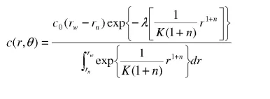
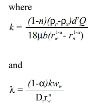
The resultant expression of the collection efficiency for the particle of size is given as

`eta _i rarr 1-exp{-lambdatheta_1}`

where

`theta_1 rarr 2*pi *(S+L)/a`

• KOCH AND LICHT MODEL

koch and Licht(1977) collection theory recognized the inherently turbulent nature of cyclones and the distribution of gas residence times within the cyclone. koch and Licht describe particle motion in the entry and collection regions with the additional following assumptions.

The tangential velocity of the particle is equal to the tangential velocity of the gas flow that is there is no slip in the tangential direction between the particle and the gas.

The tangential velocity is related to the radius of cyclone by,

`uR^n rarr constant`

A force balance and an equation on the particle collection yields the grade efficiency `eta_i`

`eta_i rarr 1 -exp {-2[((Gtau Q)/D^3 ) (n+1) ]^^(0.5)/(n+1)}`

Where

`G rarr (8k_c)/(k_a^2 k_b^2)`

`n rarr 1-{1-(12D)^0.14/2.5} {(T+460)/530}^0.3`

`tau_i rarr (rho_pd_pi^2)/(18mu)`

G is a factor related to the configuration of the cyclone, n is related to the vortex and is `tau` relation term

• LAPPLE MODEL.

Lapple(1951) model was developed based on force balance without considering the flow resistance. Lapple assumed that a particle entering the cyclone is evenly distributed across the inlet opening. The particle that travels from inlet half width to the wall in the cyclone is collected with 50% efficiency. The semi-empirical relationship developed by Lapple(1951) to calculate a 50% cut diameter, `d_(pc)` is

`d_(pc) rarr[ (9mub)/(2piN_enu_i(rho_p-rho_g))]^0.5`

where `N_e` is the number of revolutions

`N_e rarr 1/a [h+(H-h)/2]`

The efficiency of collection of any Size of particle is given by

`eta_i rarr 1/(1+(d_(pc) /d_(p i))^2)`

EXPRESSIPON.

KEYWORDS :- DISCRETE PHASE.

DISCRETE PHASE

Discrete Phase Modelling is used when the aim is to investigate the behavior of particles from a lagrangian and discrete perspective. The difference Between Lagrangian and Euler method is that fluid behavior in Langrangian is examined based on the particle tracking of a particular flow, Whereas the fluid behavior consider in Euler based on the assumptions of a Finite Element in fluid flow path.

In Discrete Phase Modelling the continous Phase is solved using the Navier-Strokes-Equation. At the Same time, the DPM is simulated by tracking the large number of Particles, Bubbles, or Droplets passing through the calculated continous flow field. Discrete phase can exchange the Momentum, Mass, and Energy with the continous phase. The method can be made much simpler by ignoring the interaction of particles (as well as droplets and bubbles) with each other. Of Course, this can happen when the discrete phase, even with a large mass, has smaller volume (less than 10%) than the continous phases. After iteration of continous phases calculated, the particle paths are calculated and determined separately.

DPM Simulation Can be Applied as,

• CFD Simulation Particle Separator from Gas using Cyclone.
• Using Particle Droplet Combution is Two and Four-Stroke combustion Engine.
• Simulation particle settling the Gravity Body Force.
• Sand Particle Tracking in pond riverside.
• Wood Combustion Using Discrete Phases Model.

• SIMUATION

CFD follows flow of following processes.

PRE-PROCESSING.

Geometry Creation.

Mesh Generation and Quality Check.

Boundary and initial Condition Setup and choice of solver.

SOLVING

Choosing the type of Solver.

Choosing Solving Strategies (Time Step, Schemes, etc)

Solver Properties (Convergence Criteria, Relaxation, etc)

If applicable, making monitor points to understand solution accuracy.

POST-PROCESSING.

Understanding the data.

Graph Plots.

Contours,

Streamline, Vector Plots, etc.

Calculation Of Properties from the existing data.

• GEOMETRY.

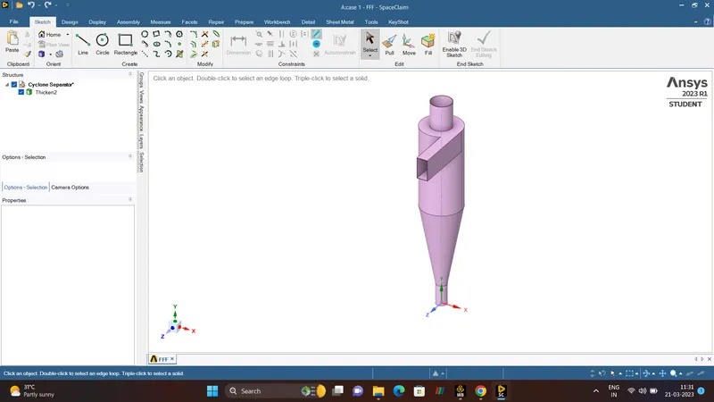
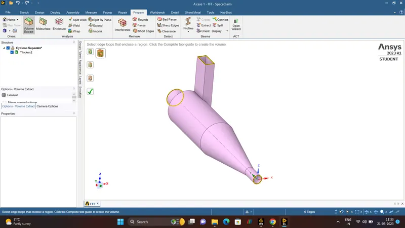
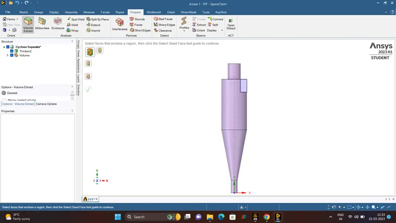
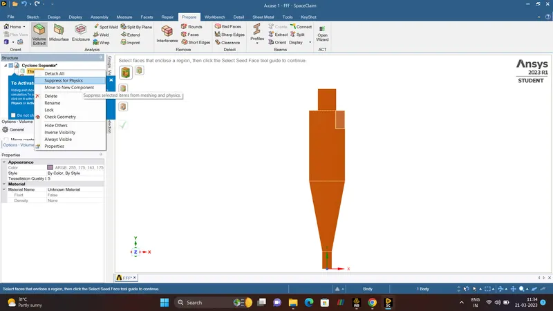
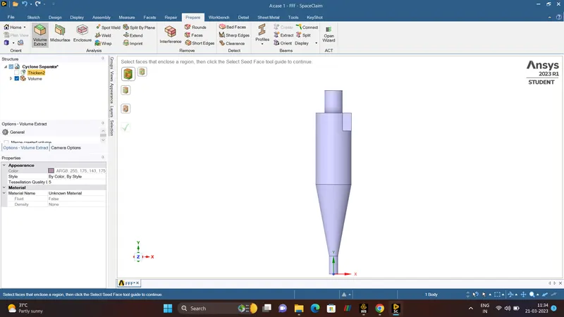
To Run the simluation of Cyclone Separator with Discrete Phase Modeling, Import the CAD model of Cyclone Separator in ANSYS-SPACECLAIM. Extract the fluid Volume by Selecting the Inner edges of Cyclone Separator(INLET, and OUTLETS). VOLUME EXTRACT `rarr`EDGE SELECT TOOL `rarr`SELECT - INLET and OUTLETS. The Purpose of Volume Extract is to Create a Soild based on a volume enclosed by a Single body or set of bodies. When the volume is created, the bodies used to generate the volume are temporarily Transparent. Then Hide the Geometry and Supress for PHYSICS is done, and finally the save the geometry.

• MESHING.

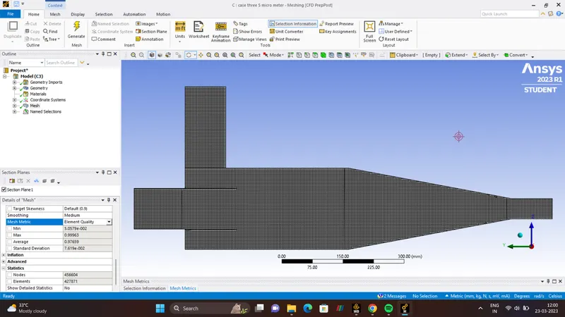
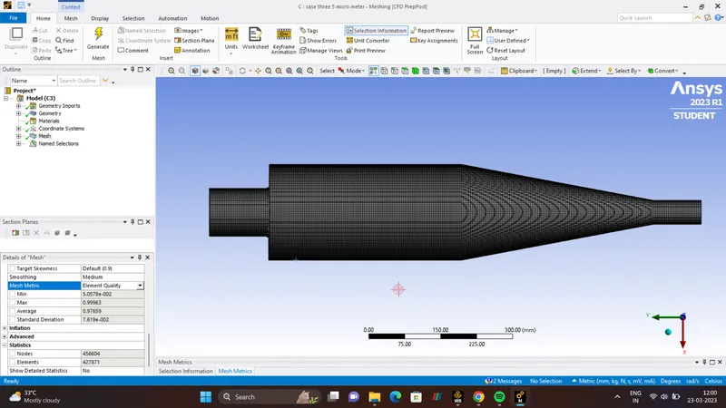
A Mesh is a network that is formed of cells and points. It can have almost any shape in any size and is used to solve the PDEs (Partial Differential Equation). Each cell of the mesh represent an individual solution of equation which, when combined for the whole network, results in a solution for entire mesh.

Why do we need Mesh?

Solving the entire object without dividing it into smaller pieces can be impossible because of complexity that is within the object. Holes, comes and angles can make it exteremly difficult for solvers to obtain solution. Small cells, on the other hand are comparably easy to solve and therefore preferred strategy. The PDEs is solved in each and every individuals cells. Hence each cell holds a local solution of discretised equation which is then combined together to develop a global solution.

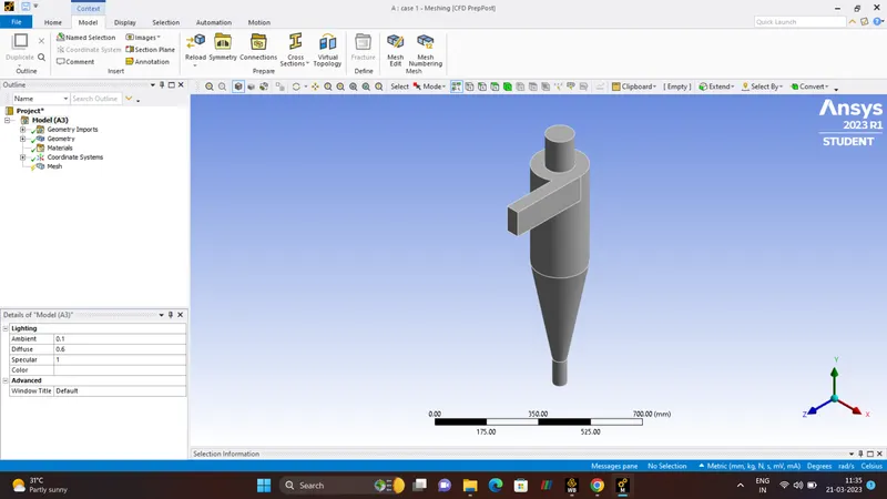
MESH`rarr`INSERT `rarr` CARTESIAN METHOD. (For Better Accuracy and Results).

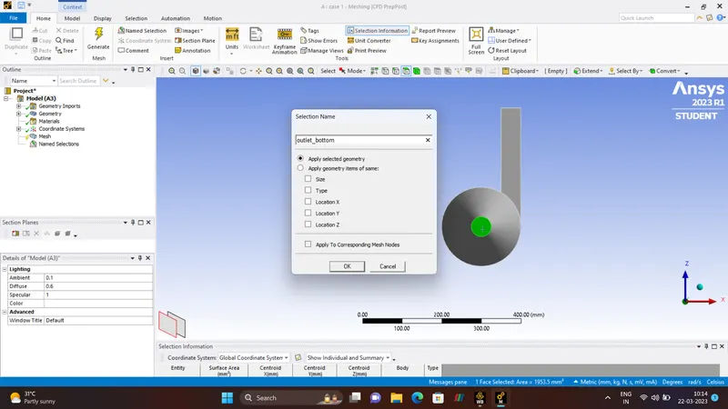
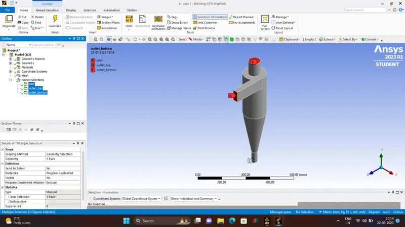
• NAME SELECTION

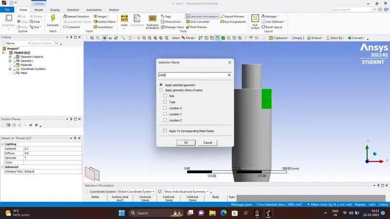
INLET.

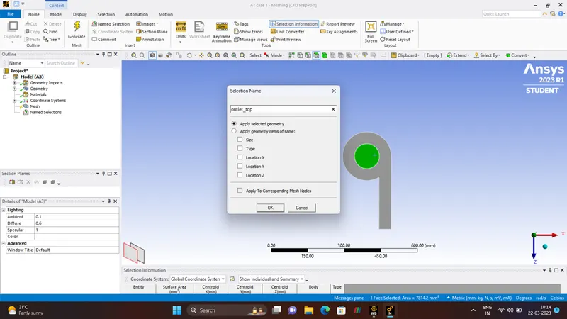
OUTLET-TOP.

OUTLET-BOTTOM.

• BOUNDARY-CONDITIONS

Boundary Condition pertain to the field of computational mechanics where we initialize the study with certain conditions. When we translate the problem to the computational domain, we assign different conditions to diiferent aspects of the domain. In layman's term, boundaries represent the physical bound and different components of computational domain which we initialize the study. We patch values of the certain flow properties on these boundaries, for instance it can be VELOCITY/PRESSURE/TEMPERATURE etc. Through which can start the iterative process of solving the problem.

• SETUP.

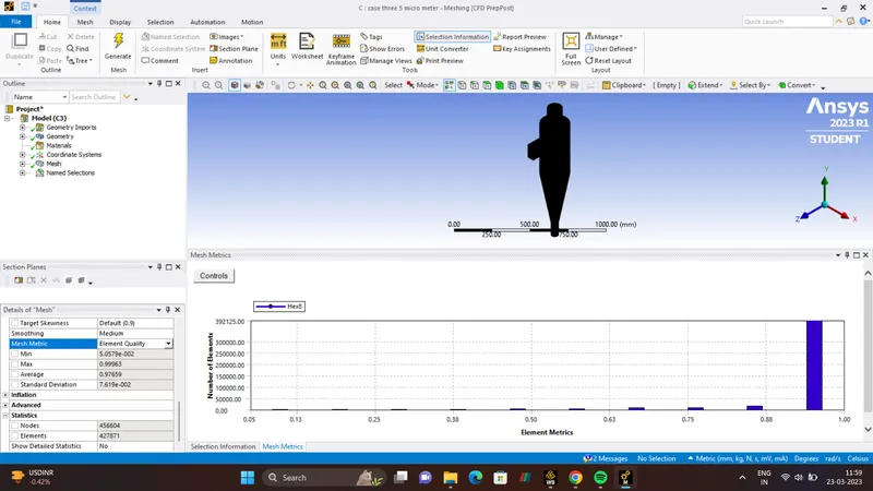
NUMBER OF ELEMENTS	427871
NUMBER OF NODES	456604
SIMULATION	STEADY-STATE-SIMULATION
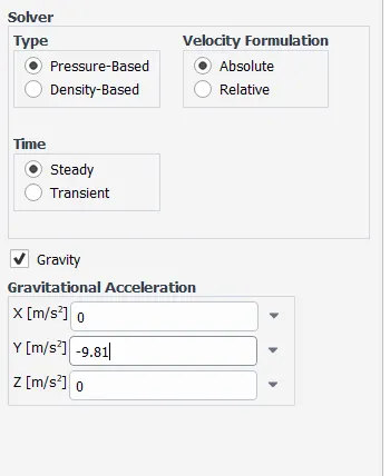
GRAVITY	ON / -9.81 `m/s^2` (Y-axis)
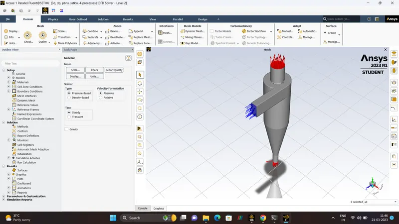
SOLVER	PRESSURE-BASED-SOLVER.
VISCOUS_MODEL	K-EPISLON `rarr` RNG `rarr`SWIRL DOMINATE FLOW
DISCRETE PHASE	ON / INTERACTION WITH CONTINOUS PHASE
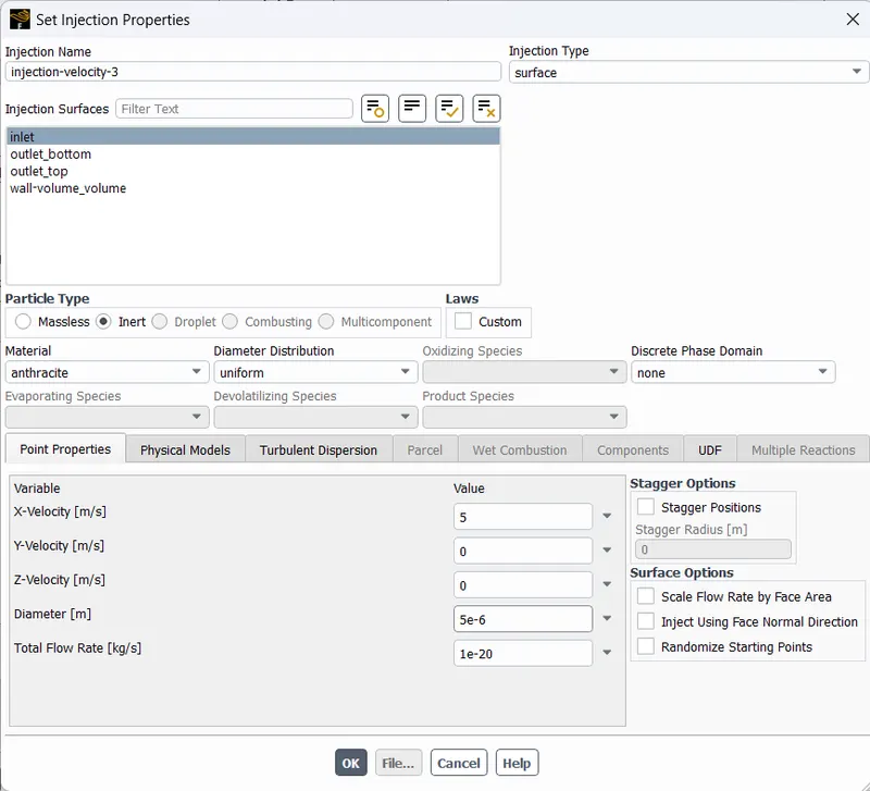
INJECTION	SURFACE`rarr`INLET`rarr`ANTHRACITE `rarr` UNIFORM
VELOCITY	3 `m/s` (CONSTANT FOR CASE 1 SIMULATIONS)
DIAMETER	1e-6 meters
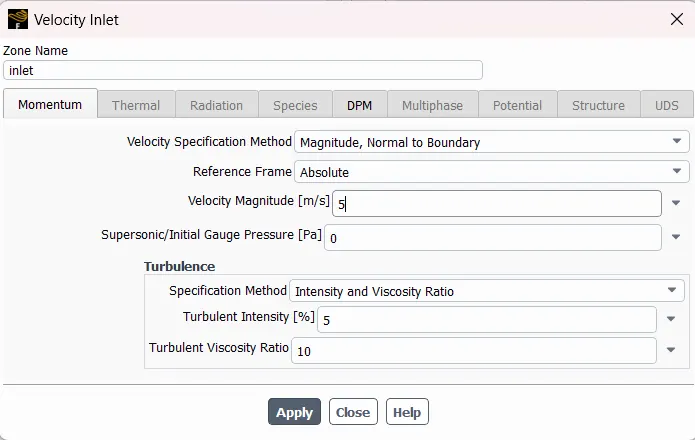
BOUNDARY_CONDITIONS	INLET`rarr`Reflect, OUTLET_TOP `rarr`Escape, OUTLET_BOTTOM `rarr` Trap
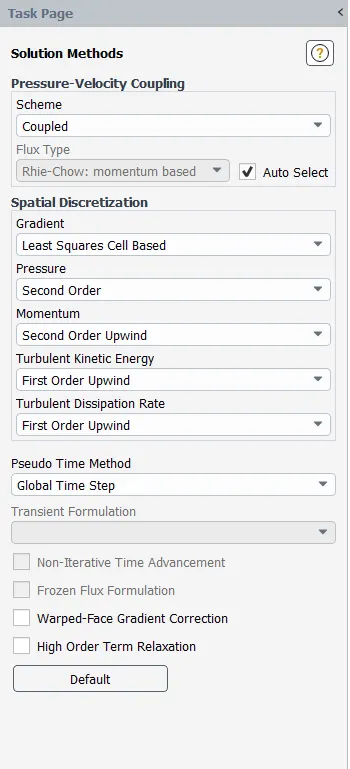
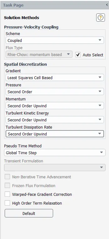
SOLUTION METHOD	SECOND ORDER UPWIND
INITIALISATION	STANDARD
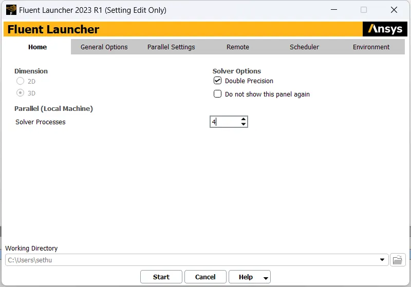
NUMBER OF ITERATION	600

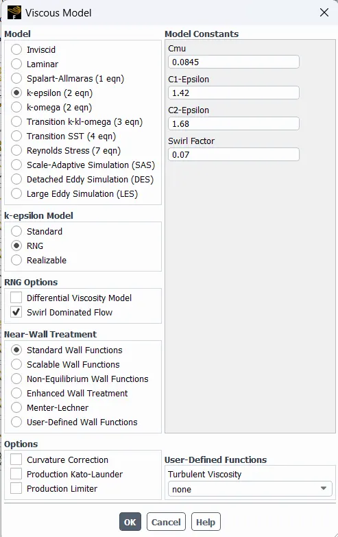
• VISCOUS-MODEL :- K-EPISLON MODEL

K-EPISLON

• K is Turbulent Kinetic Energy
• EPISLON is a Rate Of Dissipation Of Turbulent Energy.

STEADY-STATE.

• In CFD simulation, a Steady_State is Considered when all the flow properties like Temperature, Pressure, Velocity are constant.
• Steady_State Simulation computes the fully developed solution that does not change in Time.
• When Steady_State are used mean values are computed.
• Steady_State are way faster than the Transient_State Simulation.

PRESSURE-BASED SOLVER.

• Pressure Based Solver was developed for 'LOW-SPEED-INCOMPRESSIBLE' Flow (M<0.3) and midly Compressible Flow. This Solver uses Momentum and Pressure as their primary variables.

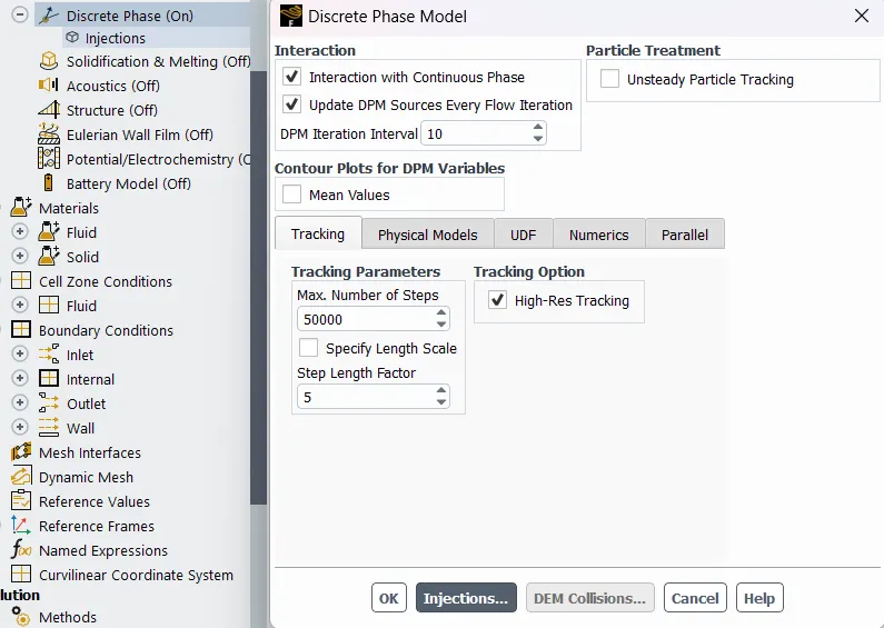
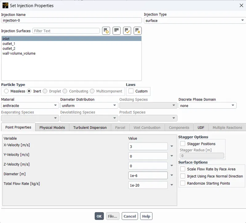
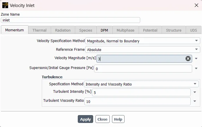
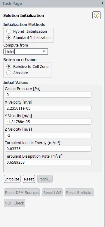
• RESULTS

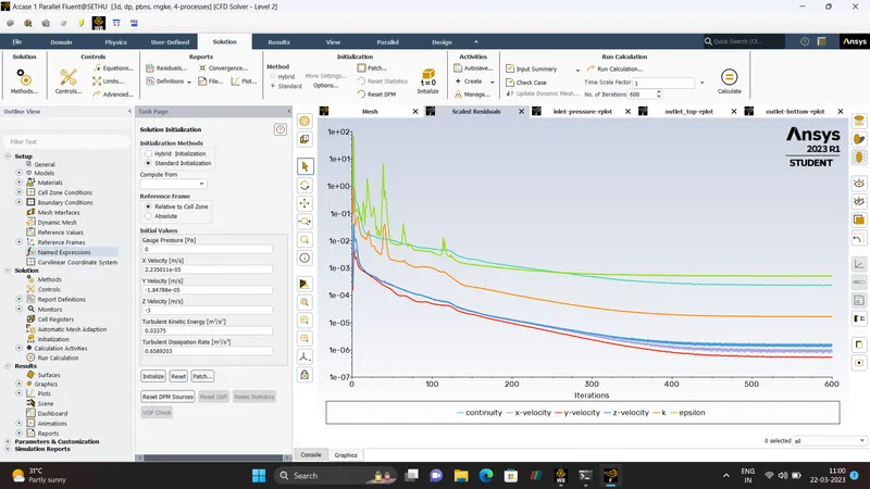
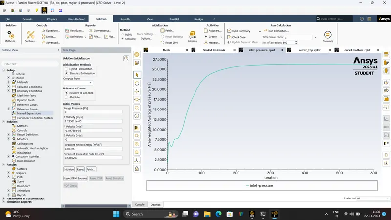
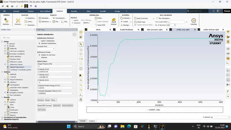
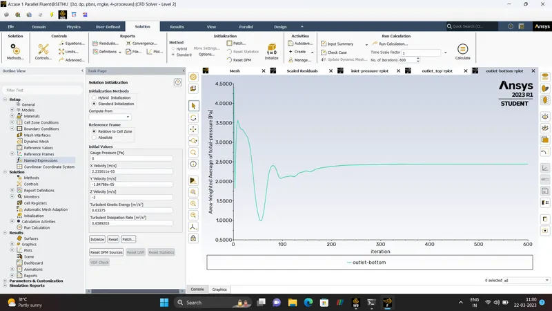
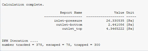
SEPRATION EFFICIENY = NUMBER OF PARTICLE TRAPPED / NUMBER OF PARTICLE TRACKED.

Calculate in % (percentage)

Seprartion Efficiency = `300/378 *100 rarr 79.36 %`

PRESSURE DROP.

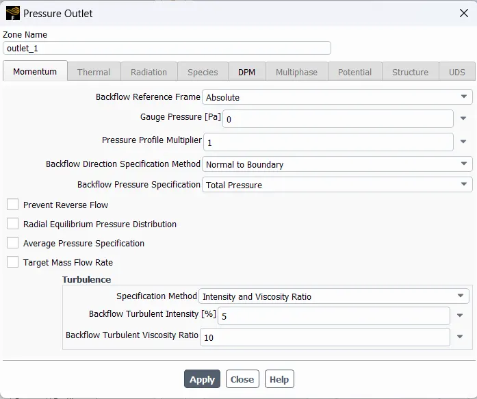
Pressure remains constant for case_one_simulation Since the velocity remains Constant as 3m/s.

Pressure Drop = Total Inlet Pressure - Total Outlet Pressure

Pressure Drop = `26.33 - (2.44 +4.34) rarr 19.55 pascal`

• CFD_POST_RESULTS.

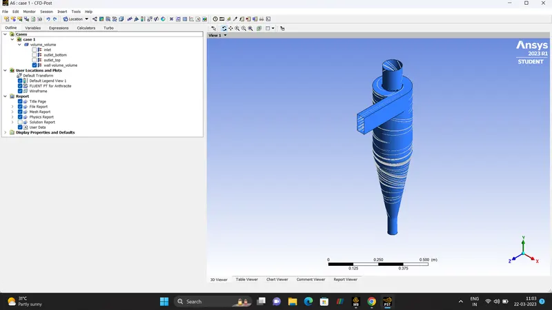
ANTHRACITE_PARTICLE_TIME.

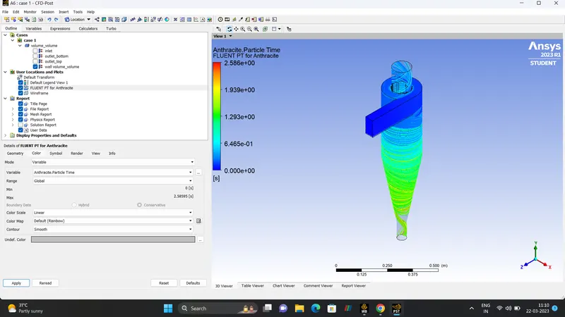
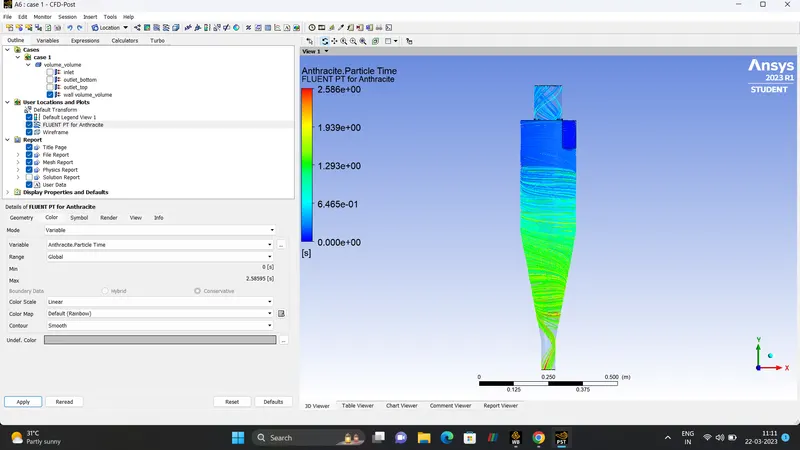
ANIMATION.

PART_ONE - CASE (2)

VELOCITY	3 m/s
DIAMETER	3e-6 meters
NIMBER OF ITERATIONS	700

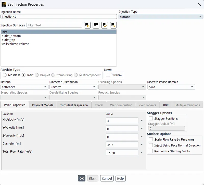
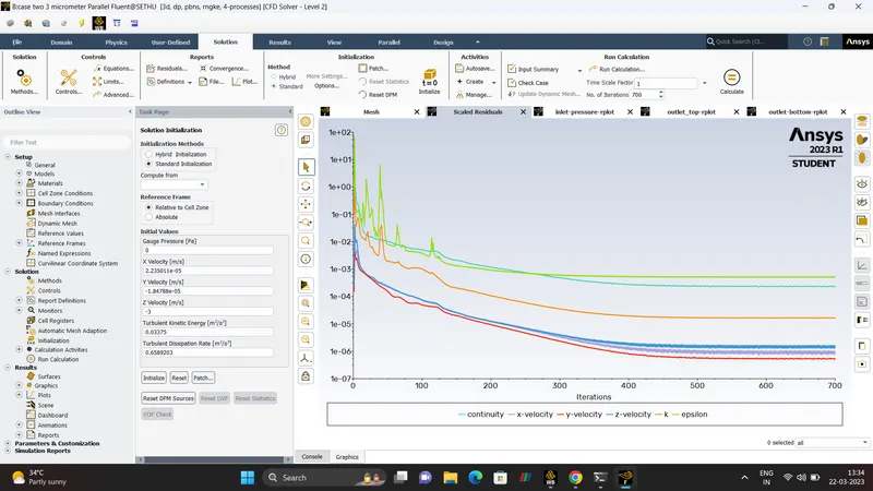
SEPRATION EFFICIENY = NUMBER OF PARTICLE TRAPPED / NUMBER OF PARTICLE TRACKED.

SEPRATION EFFICIENY = `305/378 *100 rarr 80.68 %`

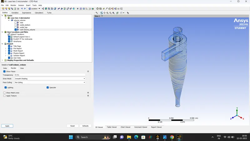
• ANTHRACITE_PARTICLE_TIME

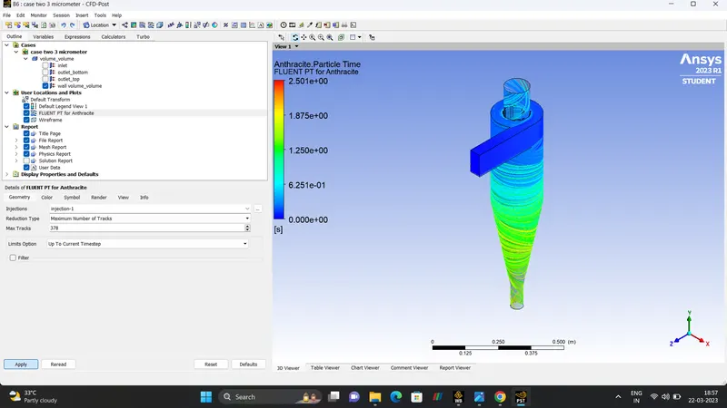
• ANIMATION.

• PART_ONE_CASE-3

VELOCITY	3m/s
DIAMETER	5e-6
NUMBER OF ITERATIONS	800

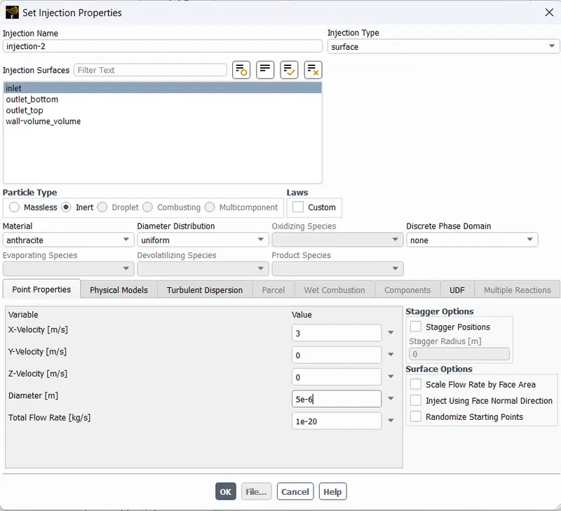
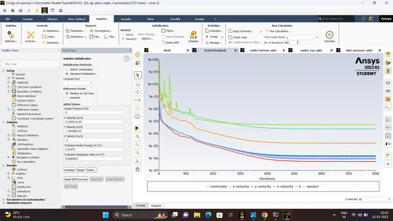
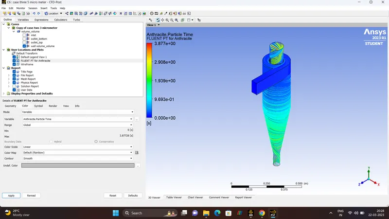
• SPERATION EFFICIENCY = 64.28%

ANTHRACITE_PARTCILE_TIME.

• PART_TWO

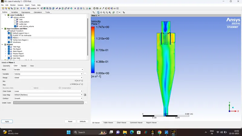
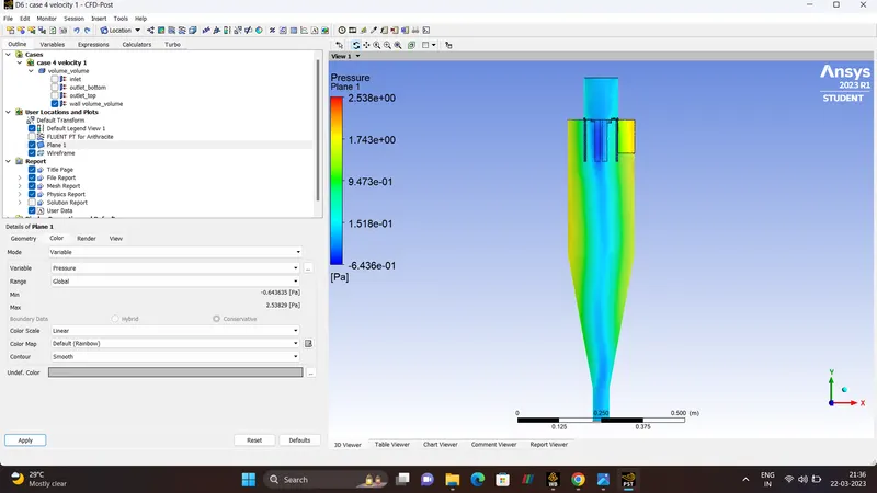
Case 1.

VELOCITY	1m/s
DIAMETER	5e-6 m (SAME FOR ALL THE CASES)
NUMBER OF ITERATIONS	600

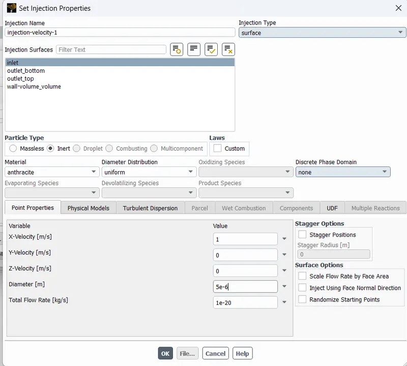
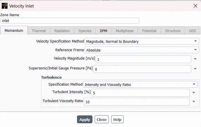
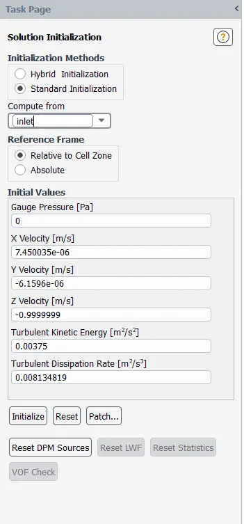
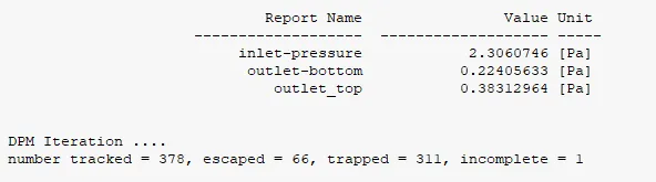
SEPARATION EFFICIENCY `311/378 *100 rarr82.27 %`

PRESSURE DROP `2.30 -(0.22+0.38) rarr 1.7 pascal`

RESULTS.

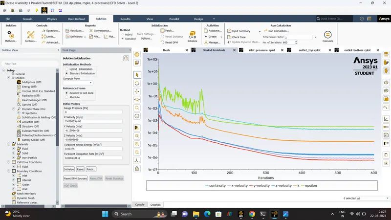
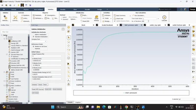
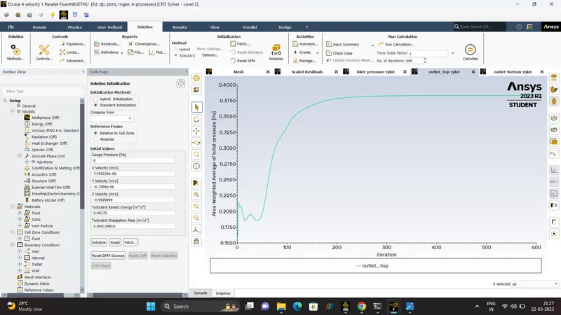
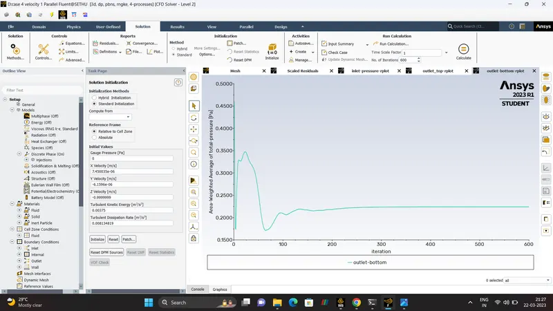
• CFD-POST.

ANTHRACITE PARTICLE TIME.

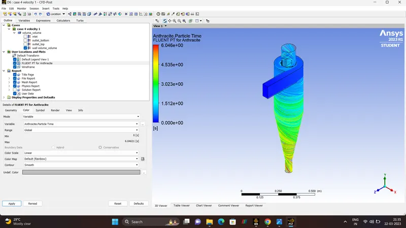
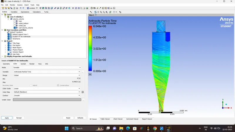
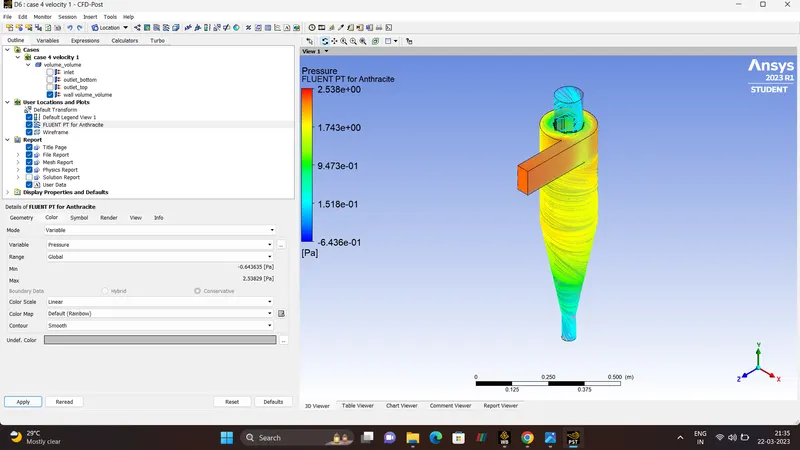
• PRESSURE

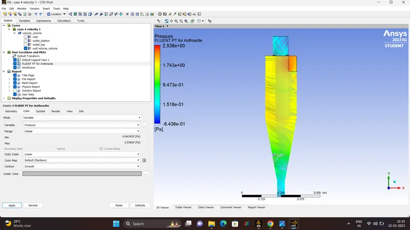
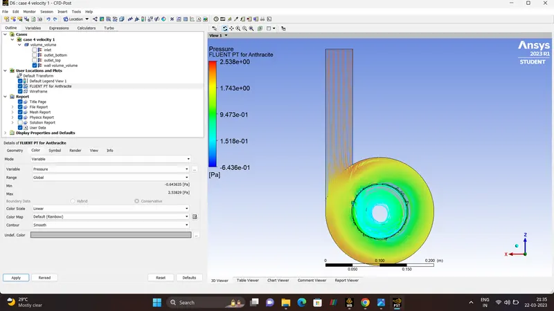
• VELOCITY

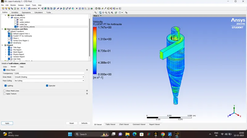
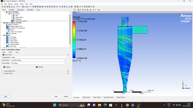
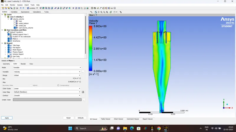
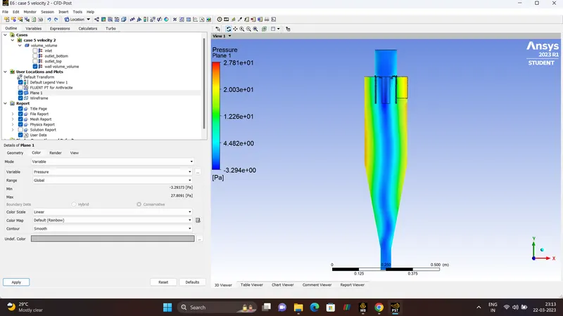
• PRESSURE/VELOCITY (PLANE)

• PART_TWO

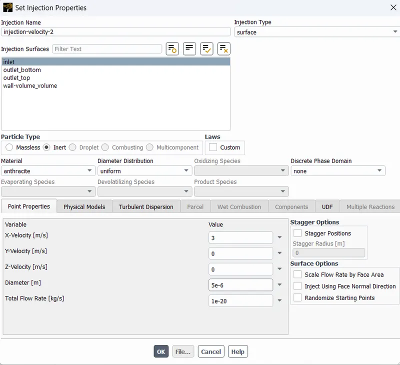
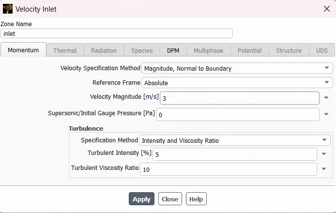
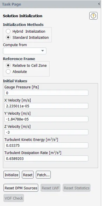
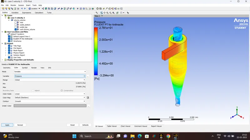
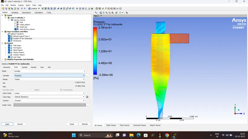
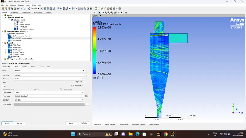
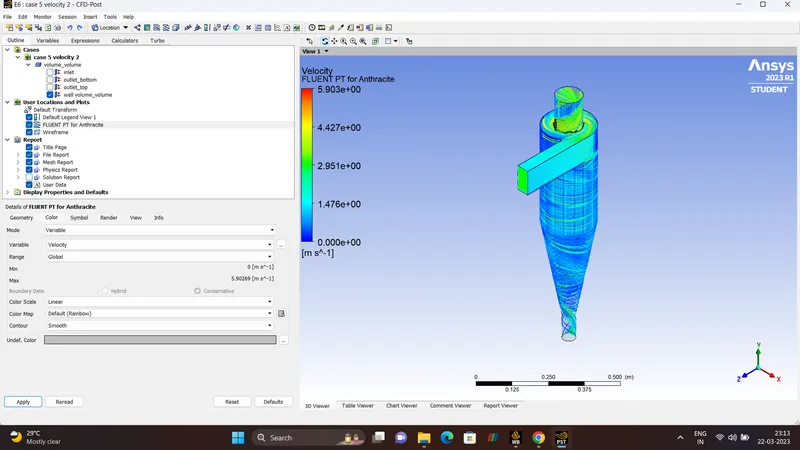
CASE 2

VELOCITY	3 m/s
DIAMETER	5e-6 m
NUMBER OF ITERATIONS	700

RESULTS

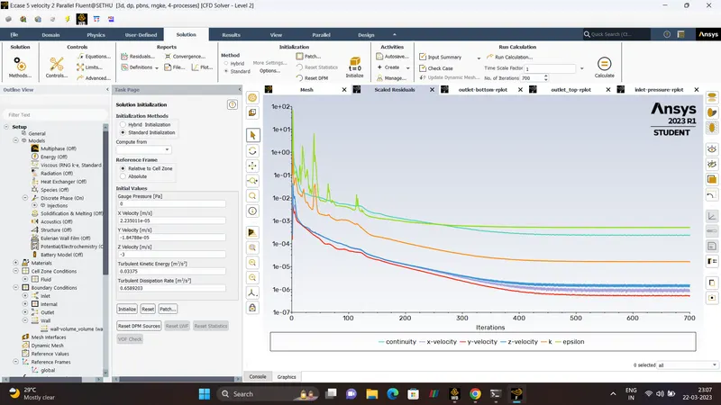
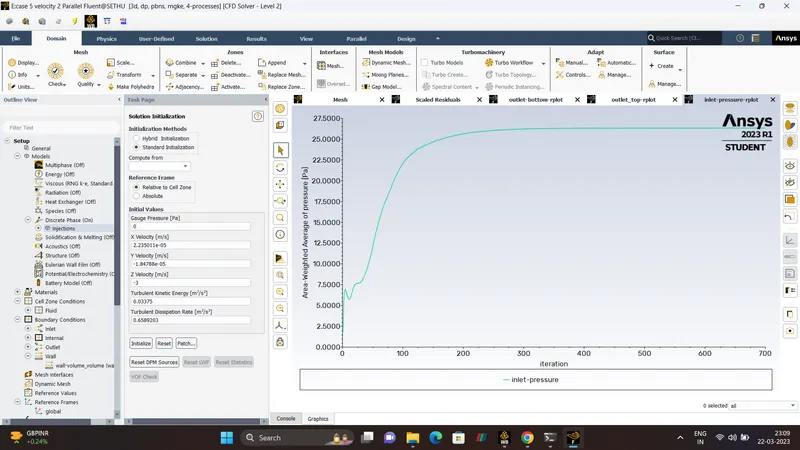
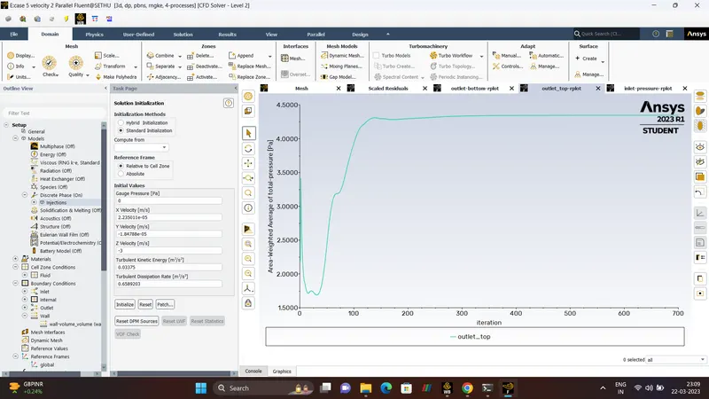
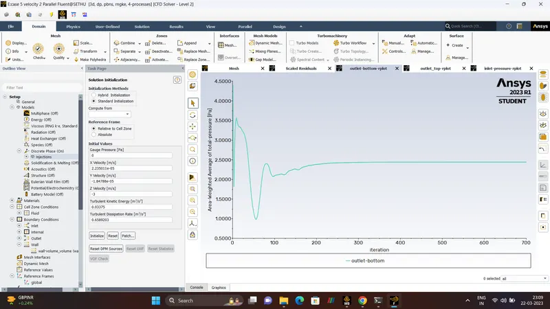
SEPARATION EFFICIENCY = 64%

• CFD-POST

ANTHRACITE PRATICLE TIME

• 

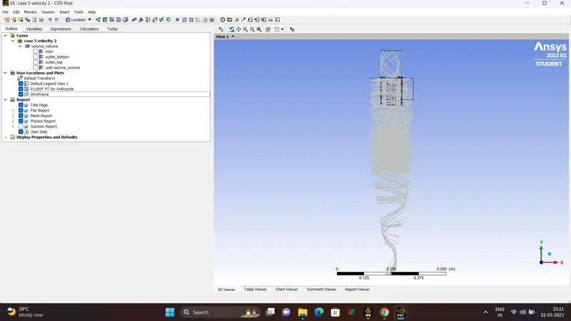
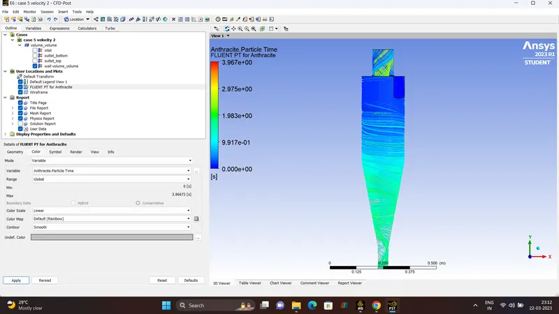
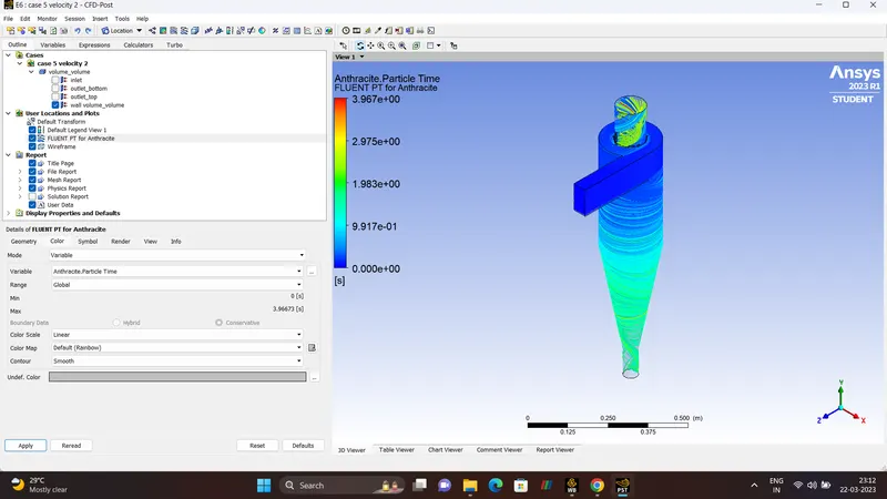
• PRESSURE

• VELOCITY

• VELOCITY/PRESSURE PLANE

• ANIMATION

PRESSURE, VELOCITY

PART_THREE

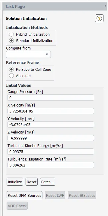
VELOCITY	5 m/s
DIAMETER	5e-6
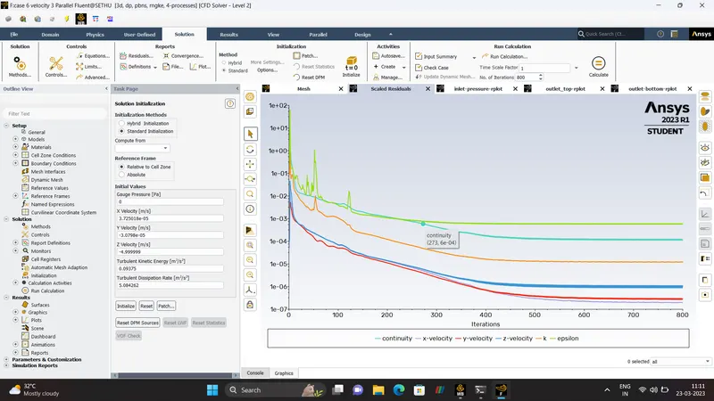
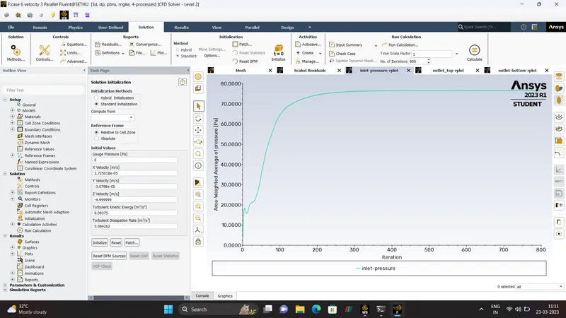
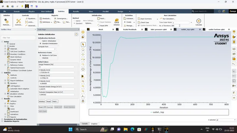
NUMBER OF ITERATIONS	800

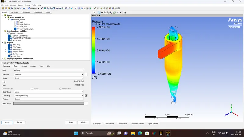
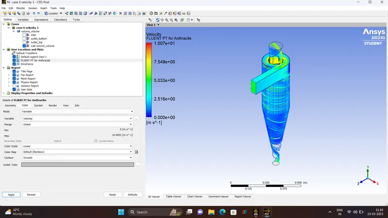
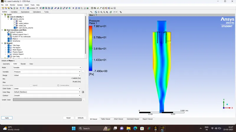
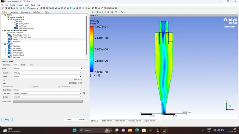
• RESULTS

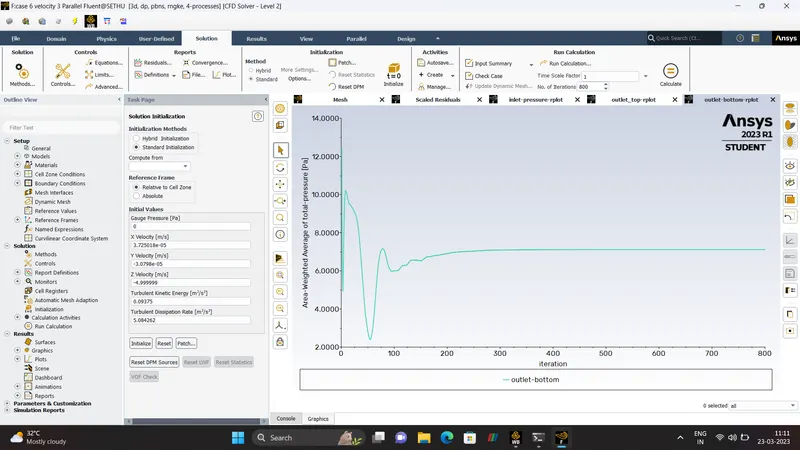
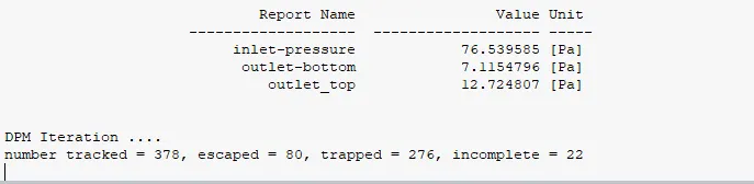
SEPARATION EFFICIENCY = 73 %

• ANTHRACITE-PARTICLE-TIME.

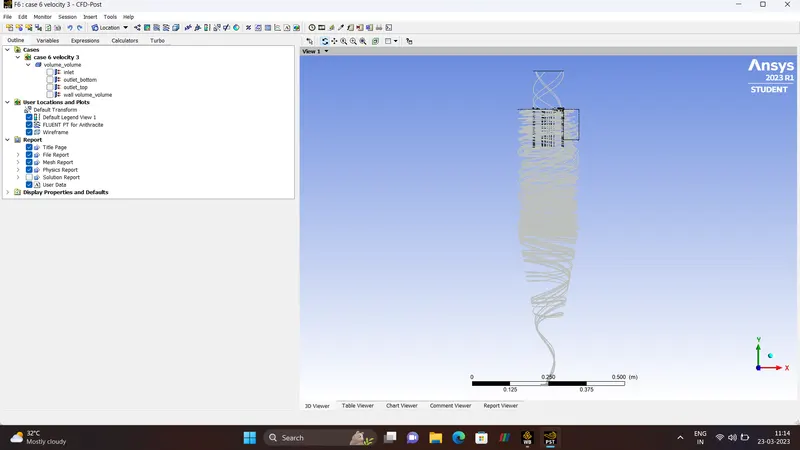
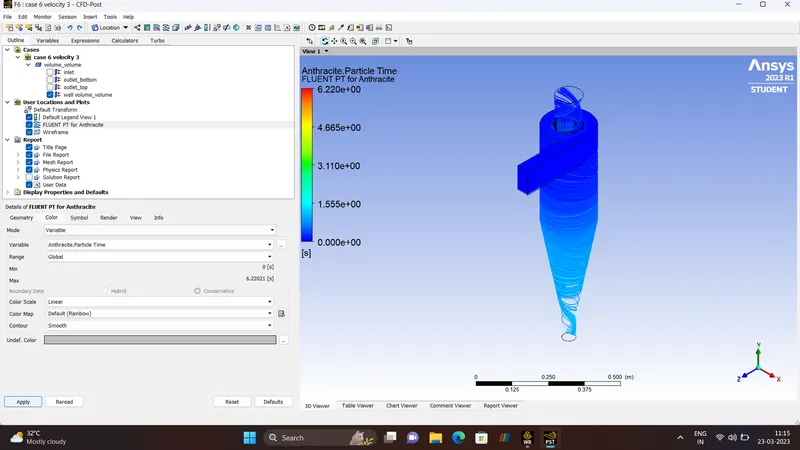
• PRESSURE & VELOCITY

• PRESSURE & VELOCITY MIDPLANE

• ANIMATION

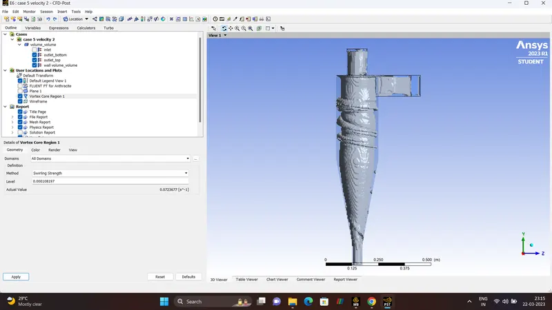
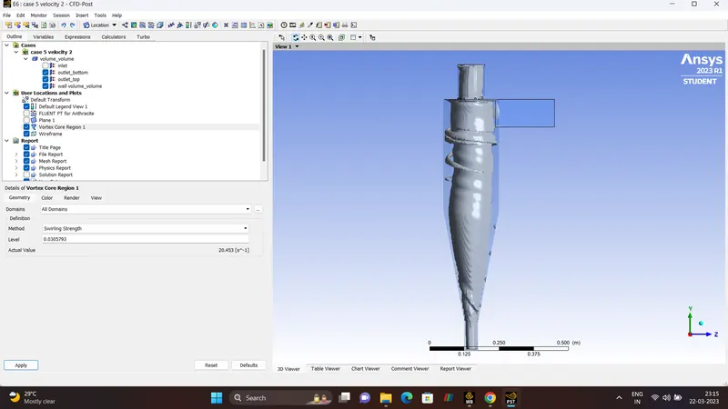
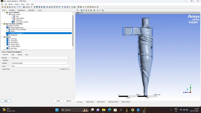
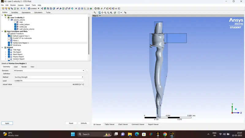
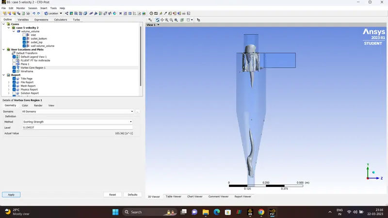
VORTEX CORE REGION.

CONCLUSION.

• Let us Conclude from the above Simulations that four empirical model and cyclone separator efficiency is been calculated.
• The efficiency of Cyclone Separator is directly propontional to the flow velocity of particulate the higher velocity Higher efficiency.
• As the particle size increase, Separator efficiency increases. As the velocity increases separator efficinecy increases.
• Finally the solutions are convergence and hence satisfied.