Week 8 - Simulating Cyclone separator with Discrete Phase Modelling
Aim :- To perform analysis on cyclone separator and calculate the separation efficiency and pressure drop.
Empirical models used to calculate the cyclone separator efficiency
1. IOZIA AND LEITH MODEL
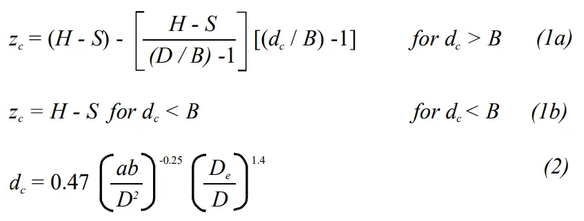
Iozia and Leith (1990) logistic model is a modified version of Barth (1956) model which is developed based on force balance. The model assumes that a particle carried by the vortex endures the influence of two forces: a centrifugal force, Z, and a flow resistance, W. Core length, zc and core diameter, dc are given as
. LI AND WANG MODEL
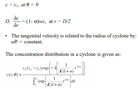
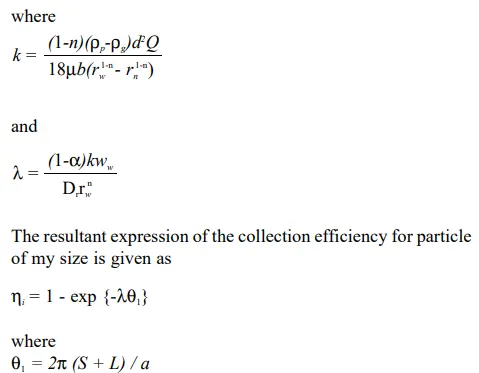
The Li and Wang (1989) model includes particle bounce or re-entrainment and turbulent diffusion at the cyclone wall. A two-dimensional analytical expression of particle distribution in the cyclone is obtained. Li and Wang model was developed based on the following assumptions:
• The radial particle velocity and the radial concentration profile are not constant, for uncollected particles within the cyclones.
• Boundary conditions with the consideration of turbulent diffusion coefficient and particle bounce re-entrainment on the cyclone wall are:
3. KOCH AND LICHT MODEL
Koch and Licht (1977) collection theory recognized the inherently turbulent nature of cyclones and the distribution of gas residence times within the cyclone. Koch and Licht describe particle motion in the entry and collection regions with the additional following assumptions:
• The tangential velocity of a particle is equal to the tangential velocity of the gas flow, i.e. there is no slip in the tangential direction between the particle and the gas.
• The tangential velocity is related to the radius of cyclone by:
uRn = constant.
A force balance and an equation on the particles collection yields the grade efficiency ηi.
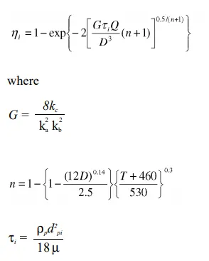
G is a factor related to the configuration of the cyclone, n is related to the vortex and τ is the relaxation term.
4. LAPPLE MODEL
Lapple (1951) model was developed based on force balance without considering the flow resistance. Lapple assumed that a particle entering the cyclone is evenly distributed across the
inlet opening. The particle that travels from inlet half width to the wall in the cyclone is collected with 50% efficiency. The semi empirical relationship developed by Lapple (1951) to
calculate a 50% cut diameter, dpc, is
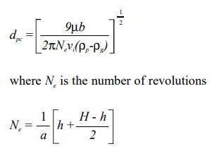
The efficiency of collection of any size of particle is given by
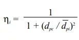
Geometry :-
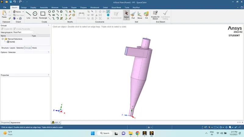
We need to extract the fluid volume by selecting the inlet and outlet edges for further use of volume.
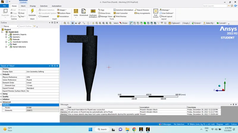
Mesh :-
Setup :-
1.Solver - Steady
2.Type - Pressure Based
3.Turbulence Model - k-epsilon > RNG > Swirl dominated > Standard wall Function
4.Gravity - -9.81 ( y direction)
5. Descrete Phase Model > Injections > surface type
6. particle type - inert
7. material - anthracite
For Case 1
particle velocity (x - velocity) - 3m/s
Diameter - varying from 1e-6 to 5e-6
Particle dia. - 1e-06
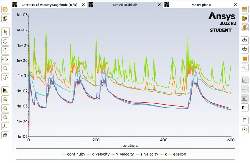
residuals :-
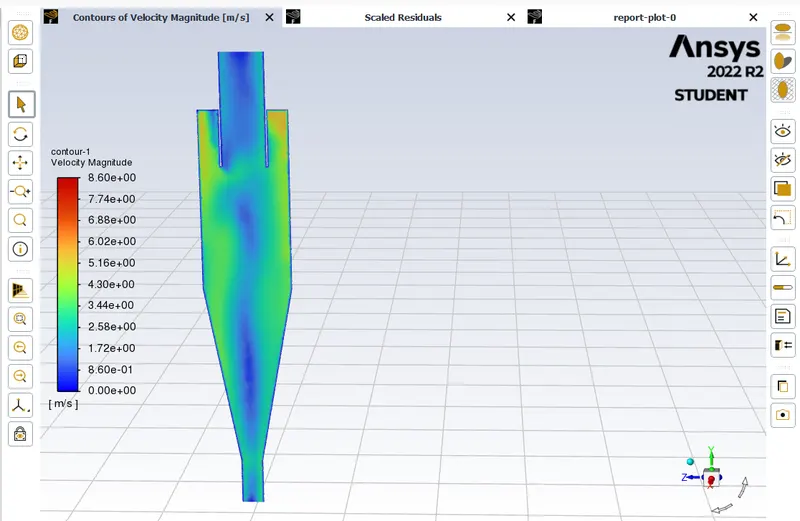
Velocity Contour :-
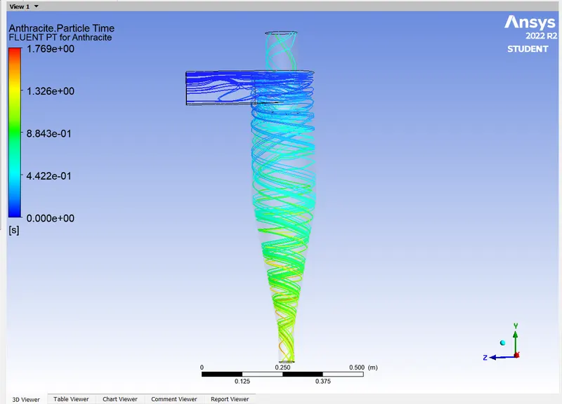
Anthracite particle time :-
https://drive.google.com/file/d/1NH9xfcb_wyohctXG5TKNPf6QCEAuxzOI/view?usp=share_link
Particle dia. - 3e-06
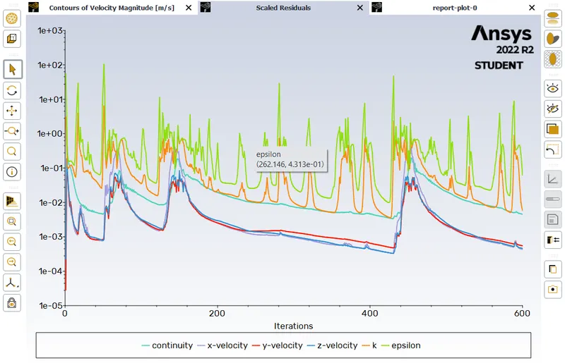
residuals :-
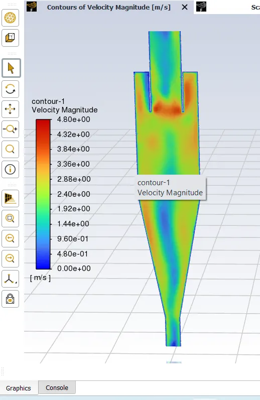
Velocity contour :-
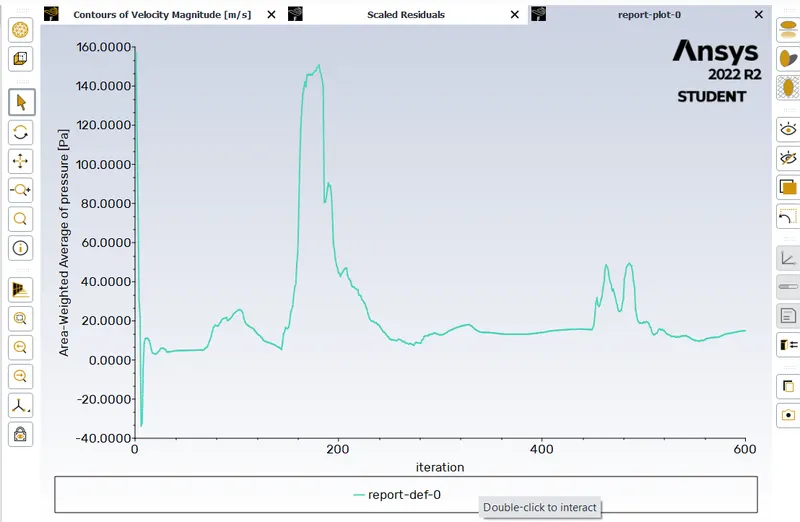
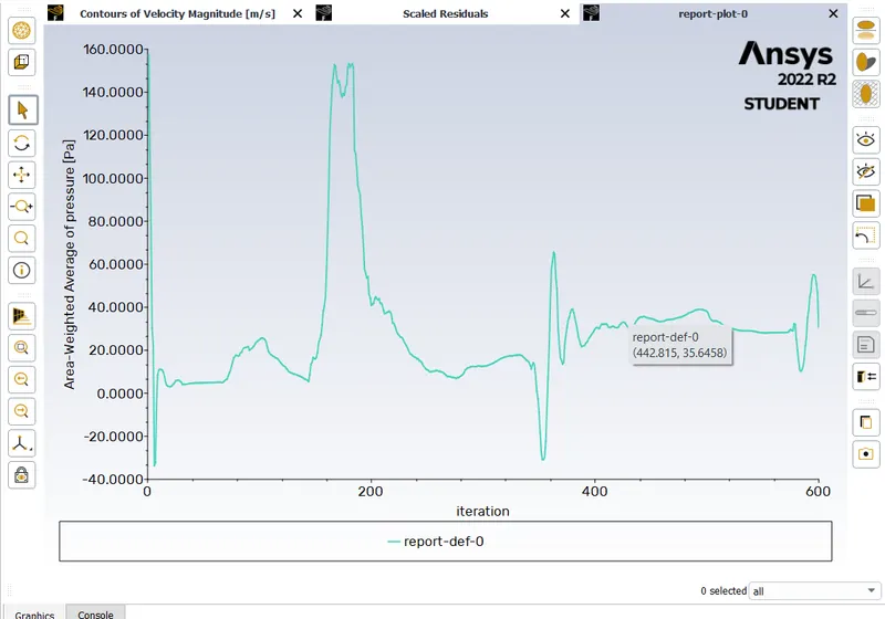
Pressure at inlet :-
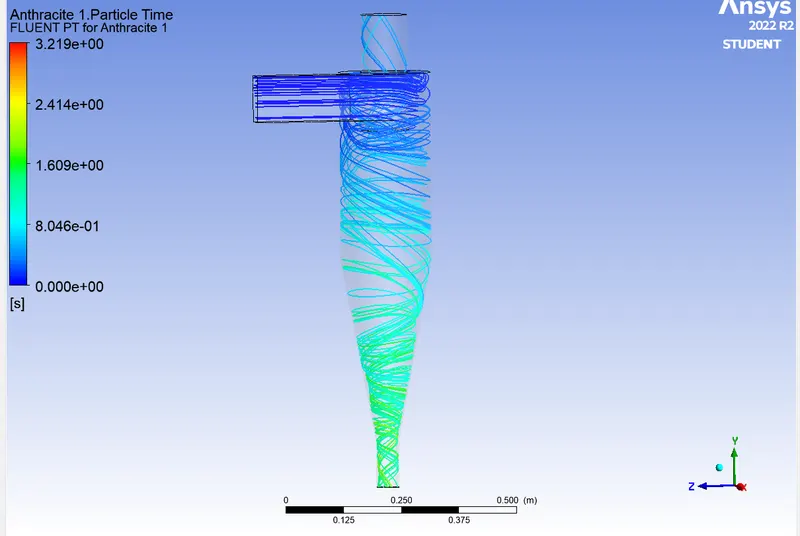
Anthracite particle time :-
https://drive.google.com/file/d/1VP7KHXkOsemLz_F_YCHxwOxWZugciyMf/view?usp=share_link
Particle dia. - 5e-06
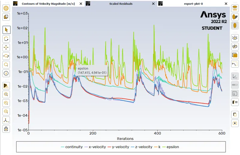
Residuals :-
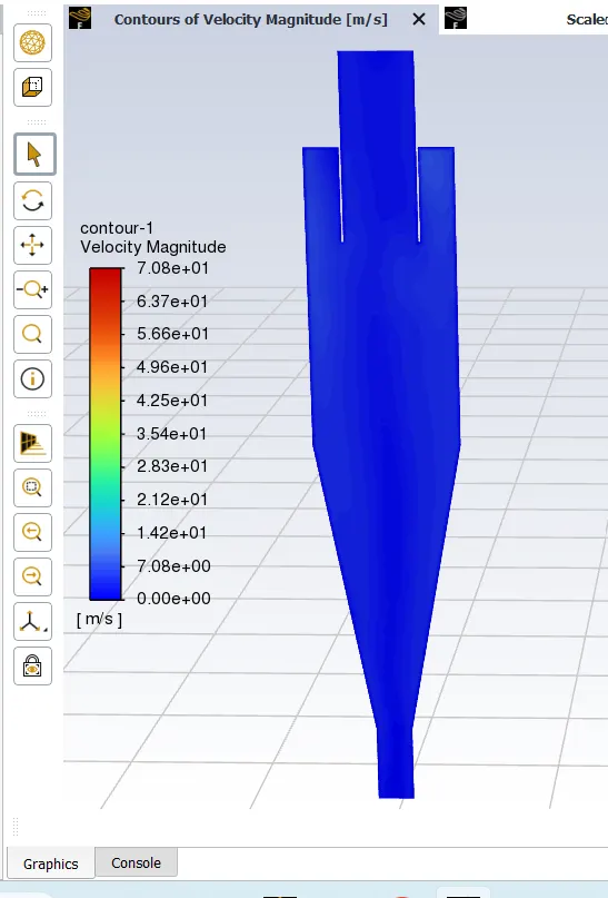
Velocity contour :-
Pressure at inlet :-
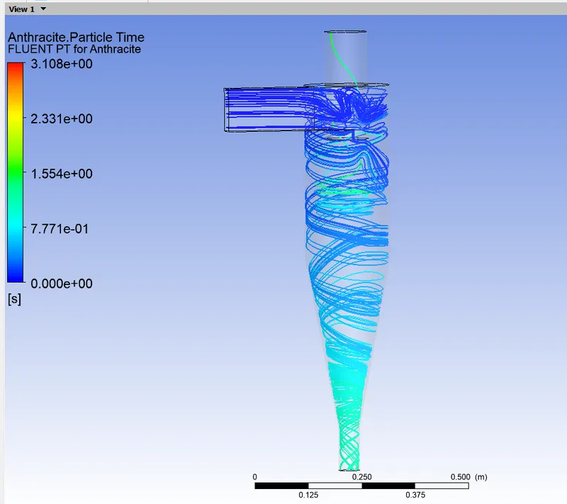
Anthracite particle time :-
https://drive.google.com/file/d/1V715q30IdftouzKhf3eUdFtITOieEizB/view?usp=share_link
Separation Efficiency:
Separation efficiency is defined as the ratio of concentration that has been removed from the feed stream to the initial concentration in the feed stream. The separation efficiency is given by the formula-
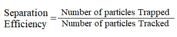
The results of the above 3 cases are tabulated below
| No. | Particle diameter (`mum`) |
Particle velocity (ms) |
Flow velocity (ms) | Number of particles tracked | Number of particles escaped | Number of particles trapped | Number of particles incomplete | Seperation Efficiency |
| 1 A | 1 | 3 | 3 | 210 | 28 | 182 | - | 0.866 |
| 2 B | 3 | 3 | 3 | 210 | 53 | 157 | - | 0.747 |
| 3 C | 5 | 3 | 3 | 210 | 17 | 193 | - | 0.919 |
For Case
particle velocity varying from (x - velocity) - 1 m/s to 3m/s
Diameter - 5e-6
Particle velocity = 1 m/s
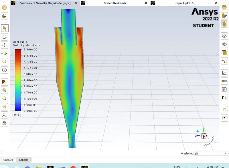
velocity contour :-
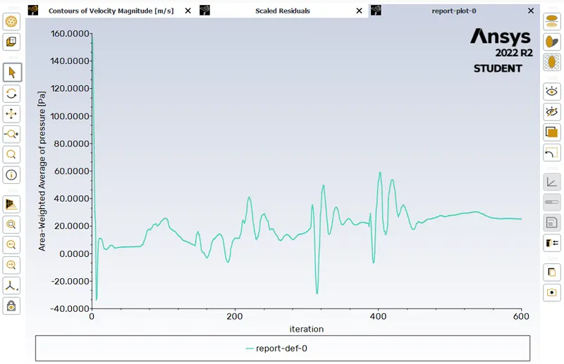
Pressure at inlet :-
Anthracite particle time :-
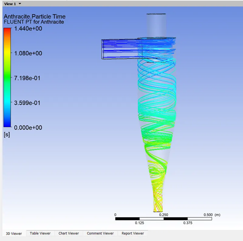
https://drive.google.com/file/d/1s3_8f9NQJeUgeeNeDUS5H-l44bcQS_XQ/view?usp=share_link
Velocity - 3 m/s
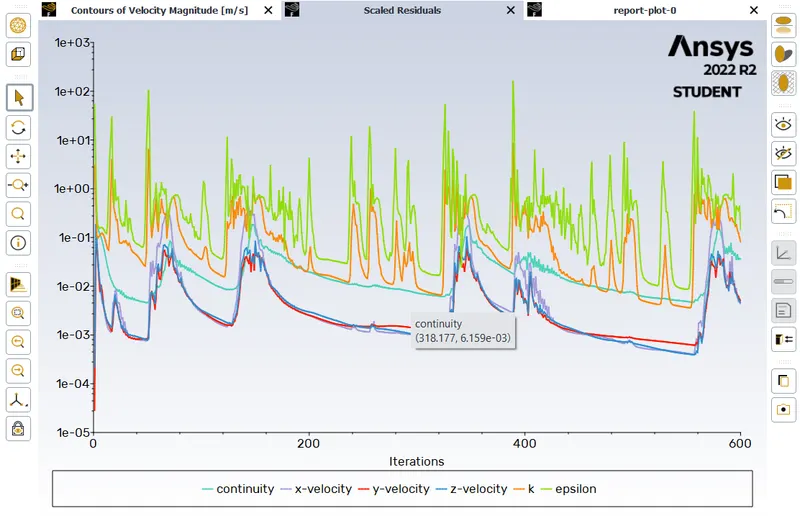
residuals :-
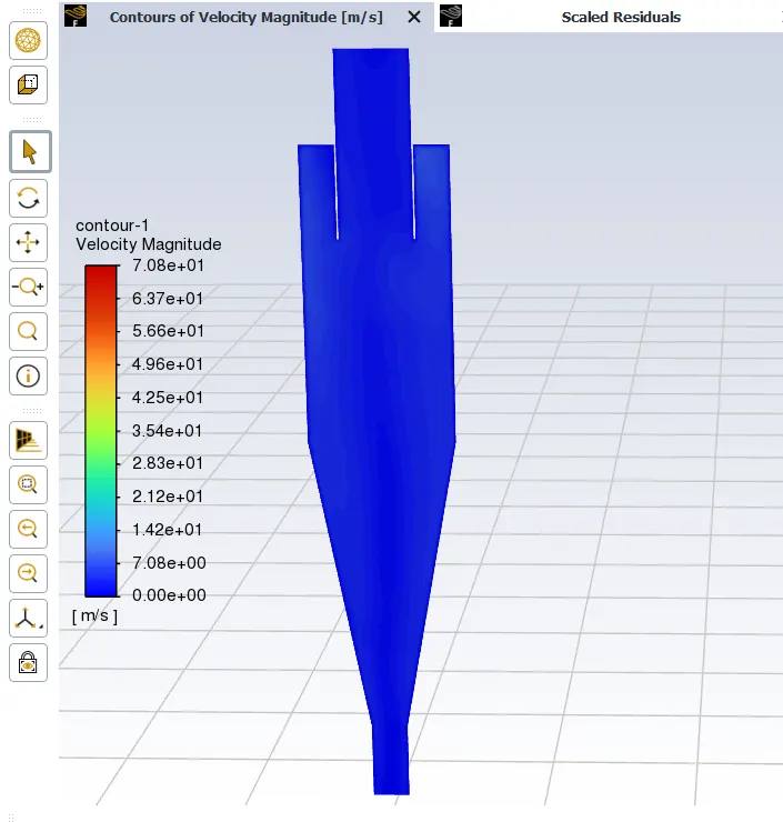
Velocity contour :-
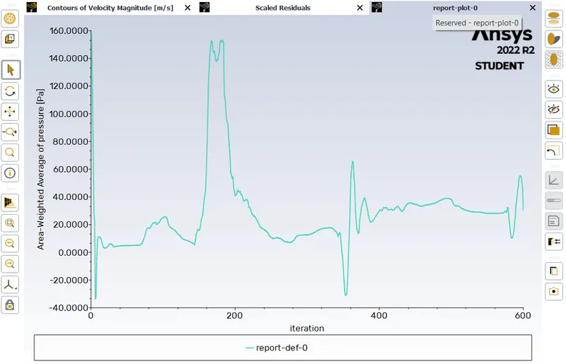
Pressure at inlet :-
Anthracite particle time :-
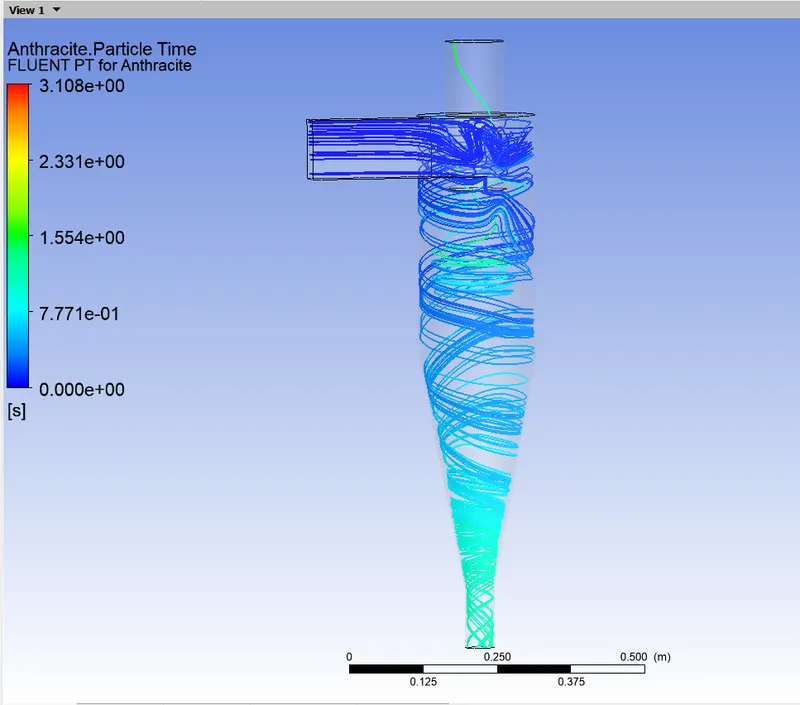
https://drive.google.com/file/d/1s3_8f9NQJeUgeeNeDUS5H-l44bcQS_XQ/view?usp=share_link
Velocity - 5 m/s
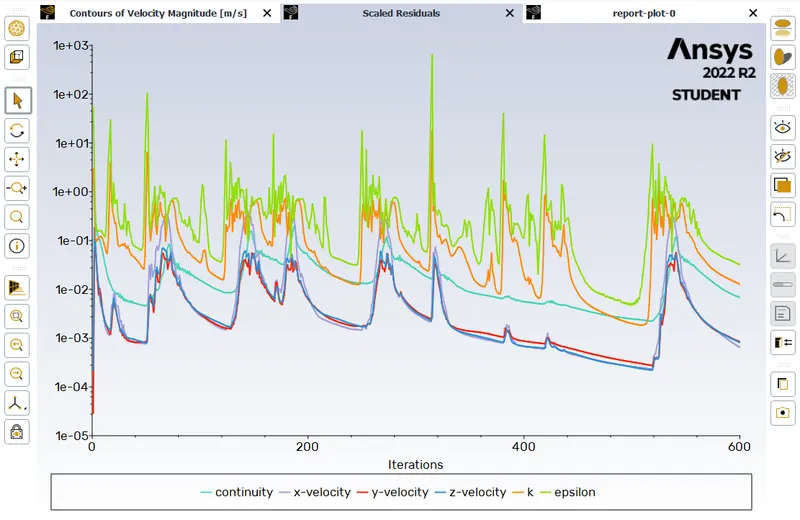
Residuals :-
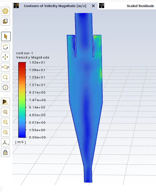
Velocity contour :-
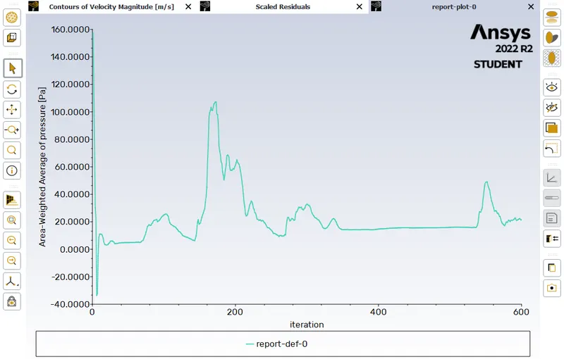
Pressure at inlet :-
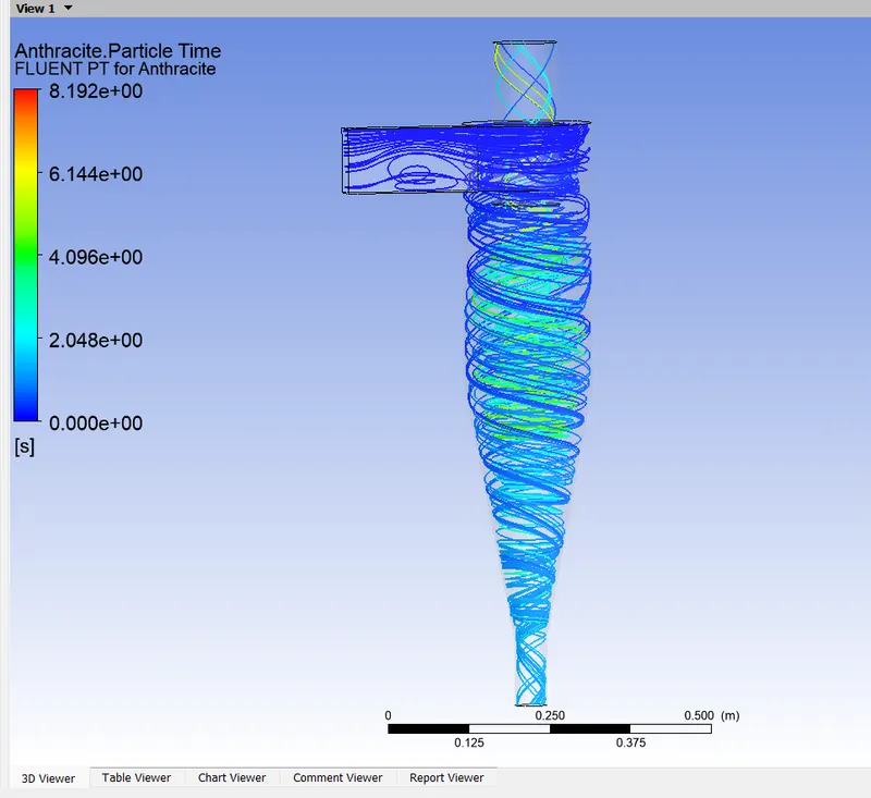
Anthracite particle time :-
https://drive.google.com/file/d/1RkI6Ojjbn6VG6KfHADlb7amh9Zo2ifXt/view?usp=share_link
The results of the above 3 cases are tabulated below
| No. | Particle diameter (`mum`) |
Particle velocity (ms) |
Flow velocity (ms) | Number of particles tracked | Number of particles escaped | Number of particles trapped | Number of particles incomplete | Seperation Efficiency | pressure drop (pa) |
| 1 A | 5 | 1 | 3 | 210 | 1 | 209 | - | 0.995 | 25.57 |
| 2 B | 5 | 3 | 3 | 210 | 17 | 193 | - | 0.919 | 30.16 |
| 3 C | 5 | 5 | 3 | 210 | 64 | 142 | 4 | 0.676 | 29.37 |
Conclusions :-
- Increasing the velocity of particle causes high pressure drop.
- As the particle diameter gradually increases the separation efficiency increases.
- As the particle velocity gradually increases and particle diameter remain same the separation efficiency increases.