Week 8 - Simulating Cyclone separator with Discrete Phase Modelling

Aim- To perform analysis on cyclone separator and calculate the separation efficiency and pressure drop using Discrete Phase Method on Ansys fluent.

Objective-

1. Write a few words about any four empirical models used to calculate the cyclone separator efficiency. 
2. To perform an analysis on a given cyclone separator model by varying the particle diameter from 1 μm to 5 μm and calculate the separation efficiency in each case. Discuss the results. [Use both the velocity's as 3m/sec.]
3. To perform an analysis on a  given cyclone separator model by varying the particle velocity from 1 m/sec to 5 m/sec and calculate the separation efficiency and pressure drop in each case. Discuss the results. [Use particle diameter size as 5 μm for all cases & keep flow velocity same as particle velocity]

Theory-

A cyclone separator is a device used to separate suspended particulate matter from the air stream with the help of centrifugal force. It consists of a cylindrical upper body with a conical lower section and two outlets are provided on top of the cylinder and at the bottom. The air enters tangentially through the inlet and then travels downwards towards the cone section forming a vortex. The increase in velocity of the air in the vortex leads to an increase in the centrifugal force of the particles separating the heavy particulate matter from the air stream. Thus, the clean air stream leaves the cyclone separator through the top outlet and heavy particulate matter is collected at the bottom.

 Empirical models used to calculate the separation efficiency of the cyclone separator:

1. Iozia and Leith model

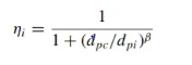
This model assumes that the particle carried by the vortex is controlled by centrifugal force and flow resistance. The collection efficiency is calculated from the below formula,

 

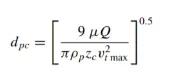
 DPC is the 50% cut size given by the barth model

2. Li and Wong model

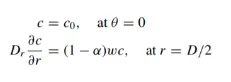
 This model includes particle re-entrainment and turbulent diffusion at the cyclone wall. This model was developed based on the assumption that the radial particle velocity and radial concentration profile are not constant for uncollected particles within cyclone. Boundary conditions with turbulent diffusion coefficient and particle re-entrainment on the cyclone wall are given below,

  

The concentration distribution in a cyclone is given,

 

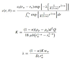
The collection efficiency for any given particle size is,

 

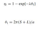
3. Kocht and Licht model

This model describes the particle motion in the entry and collection regions with assumptions that the tangential velocity of the particle is equal to tangential velocity of the gas flow and the tangential velocity and radius of the cyclone are related by .

 

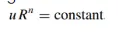
The collection efficiency is given by,

 

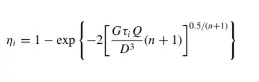
4. Lapple model

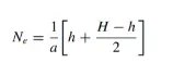
 This model was developed based on the force balance without considering flow resistance. It was assumed that the particle entering the cyclone is evenly distributed across the inlet. Lappel developed an empirical relationship to calculate 50% cut diameter and it is given by,

 

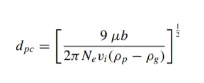
The number of revolutions is given by,

 

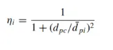
The collection efficiency of any given size of the particle is given by,

 

Geometry-

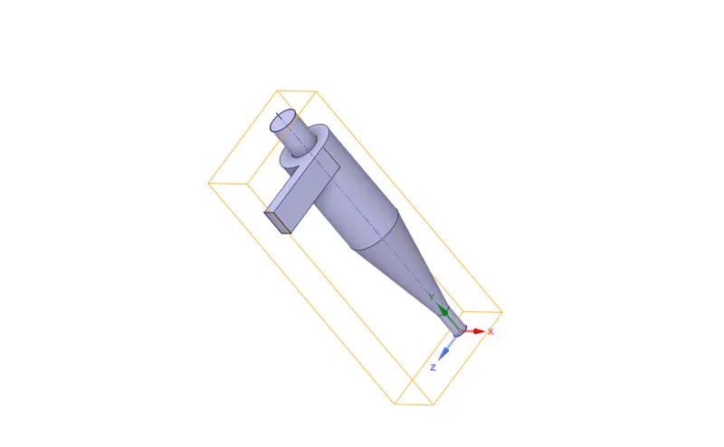
• Import the cyclone separator geometry on the space claim of ansys workbench.

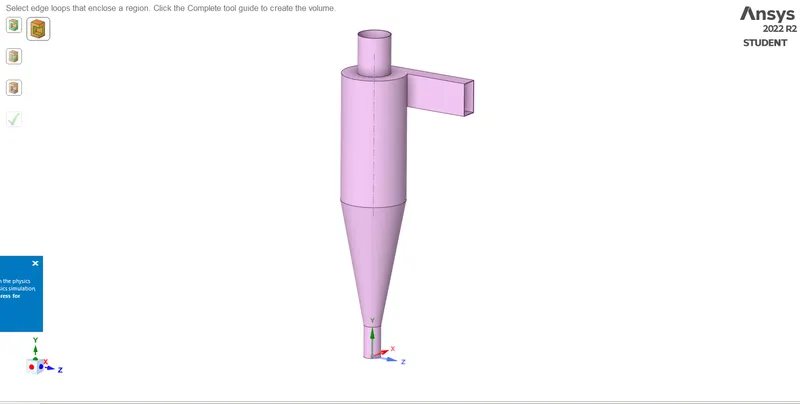
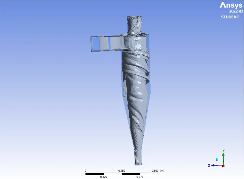
• Then analyse the geometry and perform a volume extraction method and supress the solid volume using an option ‘supress for physics’ so it cannot interfere while meshing.

Meshing-

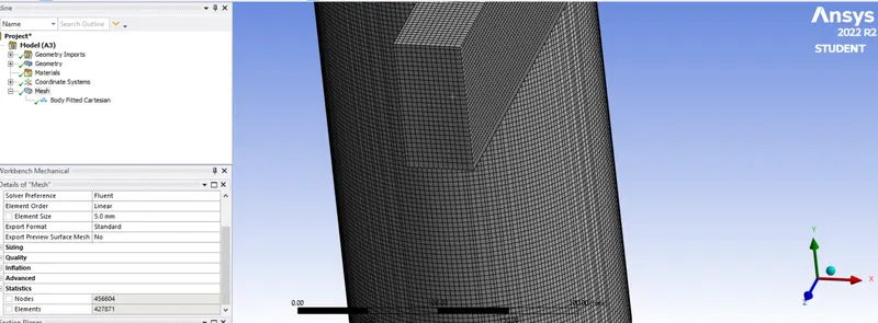
• We use here a cartesian cut method for performing the analysis because it is good in capturing the irregular geometrical entities by using cutting into smaller cells of any irregular cells any cell intersected by the boundary.
• We have use mesh element size as 5.0 mm for the refined mesh. And to capture more details of the fluent simulation.

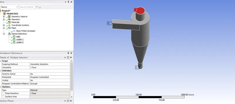
• Assign names of the faces using the named selection tool on ansys mesh.

Setup-

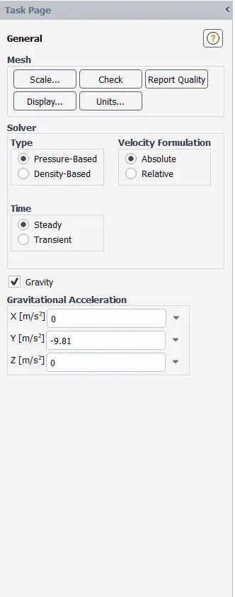
• For fluent analysis, we use here steady state time analysis and pressure-based solver with velocity formulation as absolute. And because this simulation is gravity based so gravity module has been enabled and y=9.81m/s² and X and Z are set as zero.

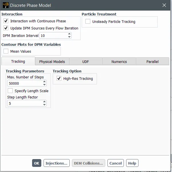
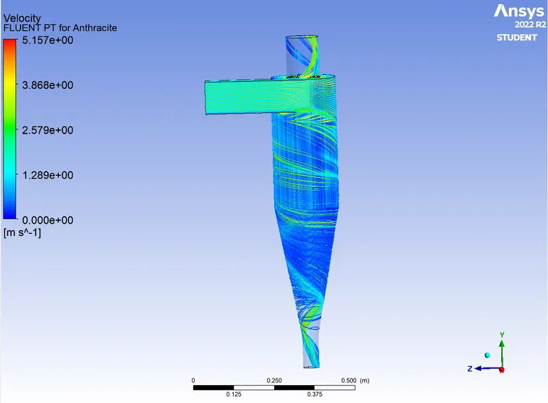
• Enable the discrete phase method and checklist the below constraints on the mentioned fig.

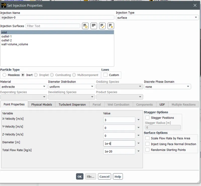
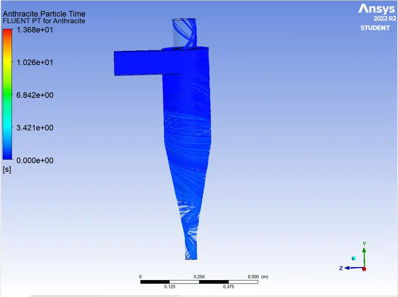
• Then plot injection properties by mentioning the name and-

                                Injection type- surface

                                Injection surface – inlet

                                Material – Anthracite

                                Diametric distribution- uniform

                                Point properties mention as --x velocity(m/s)- mentioned velocity

                                                                                    Y velocity(m/s)-0

                                                                                   Z velocity(m/s)- 0

                                                                                  Diameter(m)- according to mentioned two cases(1e-6)

                                                                                  Total flow rate – 1e-20 kg/s

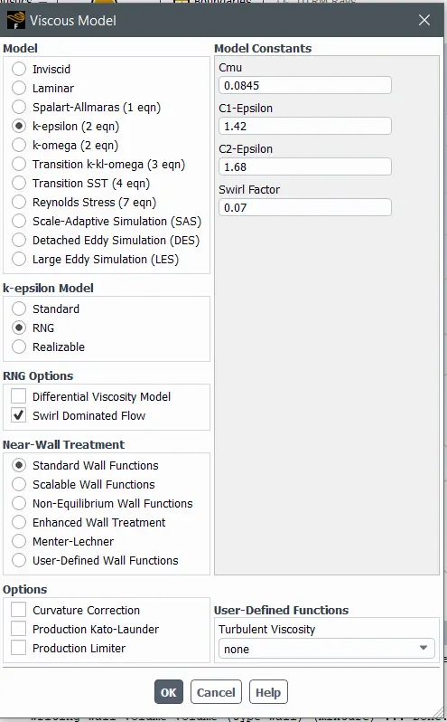
• We use viscous model as K-epsilon with RNG and swirl Dominated flow as the RNG option and with a Standard wall function as a Near wall treatment.

• Now for the boundary conditions-

Inlet------velocity=(according to the cases in m/s)     and DPM is set as “reflect”.

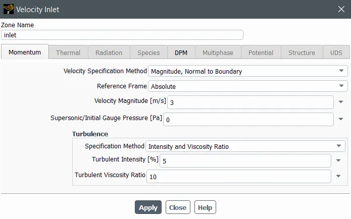
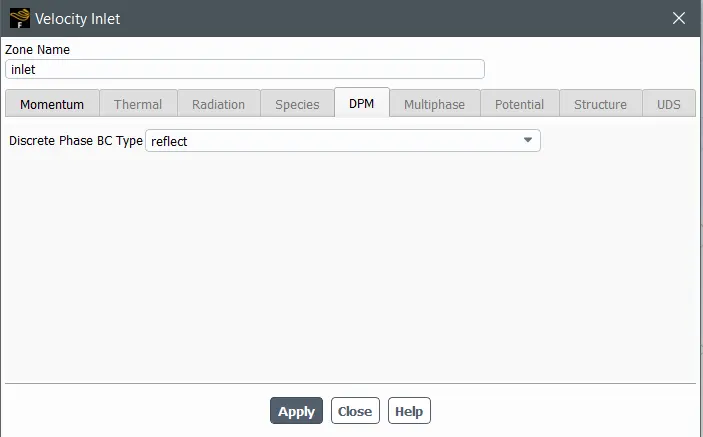
Outlet----1. Outlet-1—Pressure is to 0 pascals and DPM is set as “escape”.

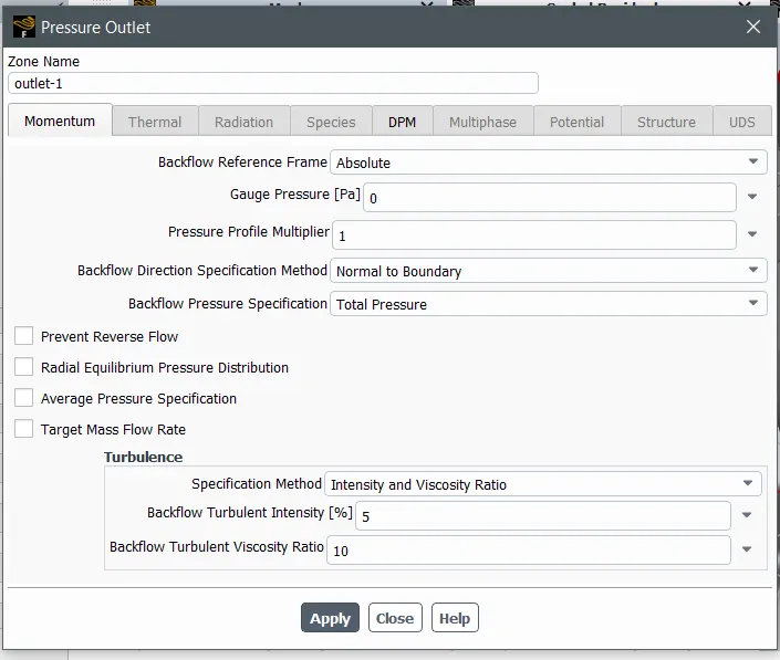
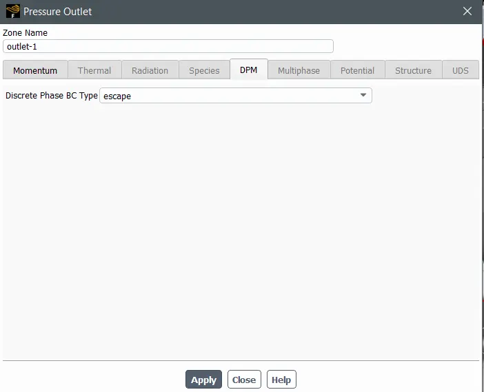
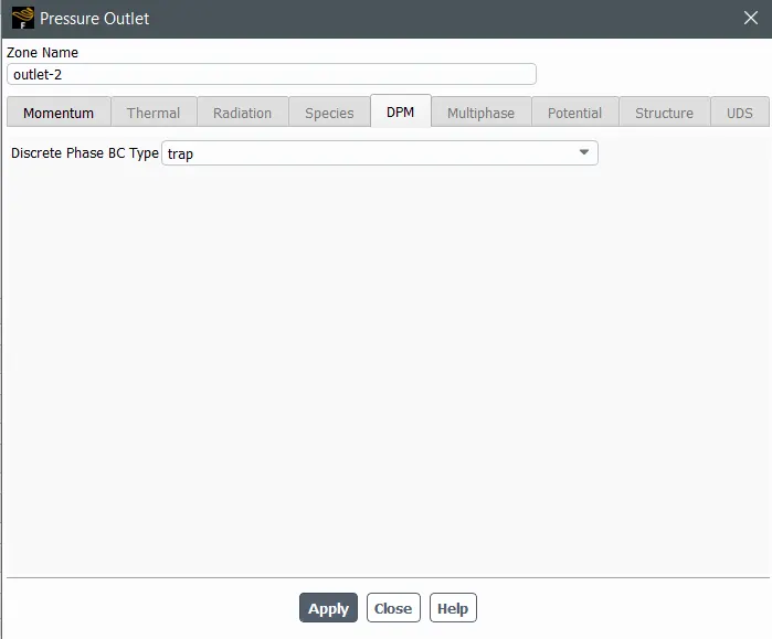
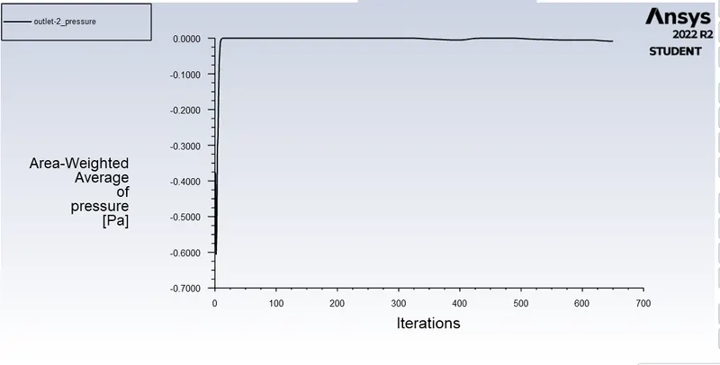
           2.Outlet-2 ----Pressure is 0 pascals and DPM is set as a “trap”.

• For Solution methods, we go with

Scheme- simple

Gradient – least square cell-based

Pressure- second order

Momentum – second order upwind

Turbulent kinetic energy- second order upwind

Turbulent Dissipation rate- second order upwind

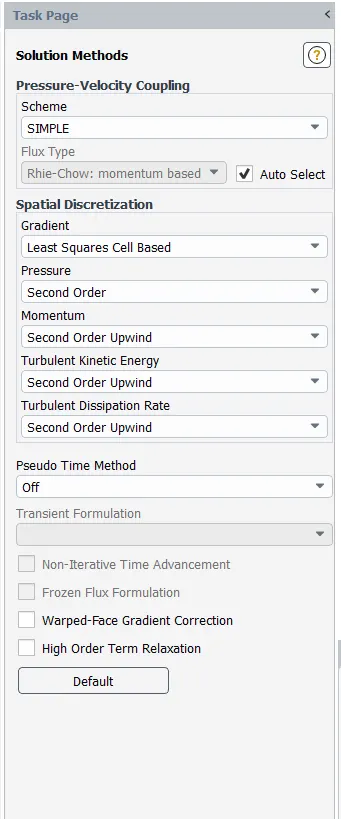
• This simulation is performed with Standard initialization with some inputs mentioned below-

Compute from- inlet

Reference frame- relative to cell zones

Gauge pressure- 0 pa

X velocity- 0m/s

Y velocity- 0m/s

Z velocity – (-ve value of inlet velocity)m/s

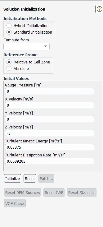
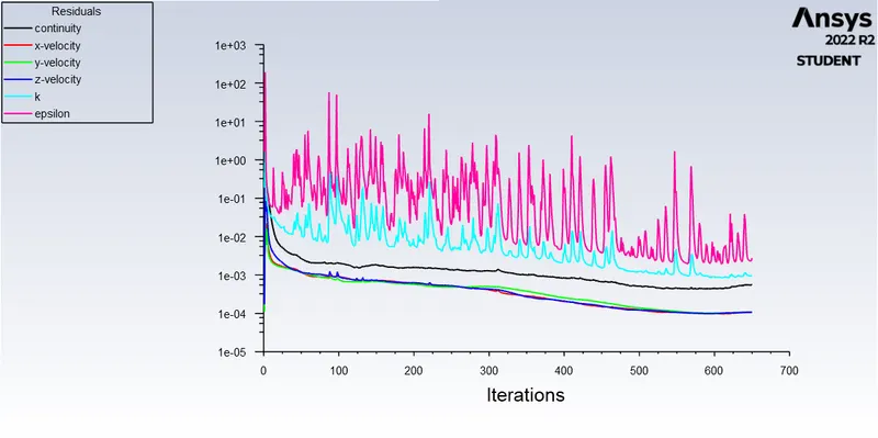
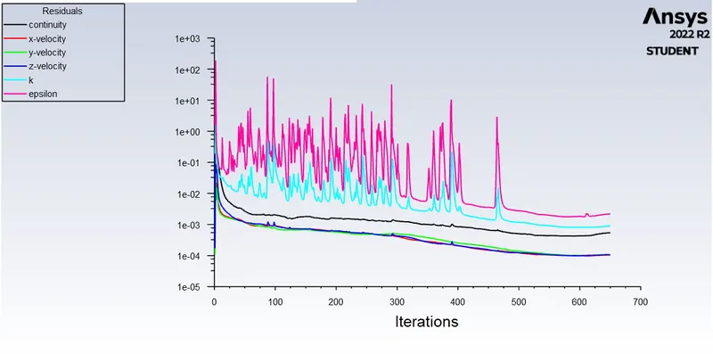
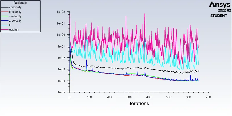
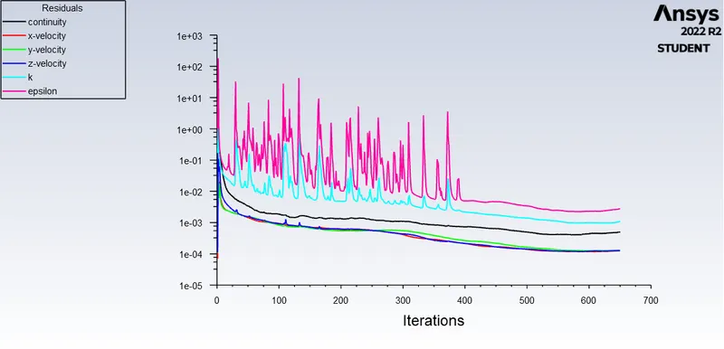
• We ran this simulation for 650 iterations.

Part-1   To perform an analysis on a given cyclone separator model by varying the particle diameter from 1 μm to  5 μm and calculate the separation efficiency in each case.

Case-i    Diameter= 1e-6 at velocity = 3m/s

 

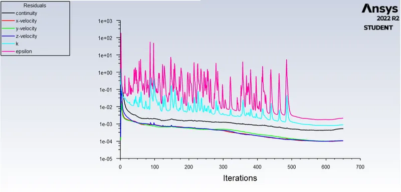
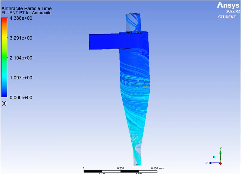
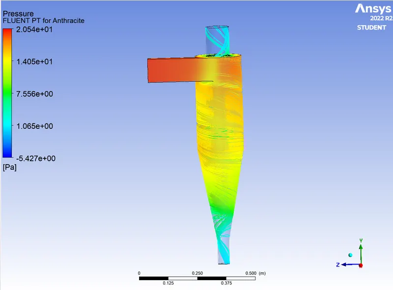
Case-ii    Diameter= 2e-6 at velocity = 3m/s

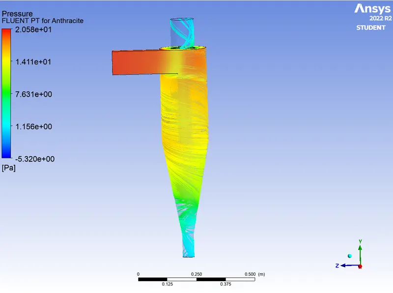
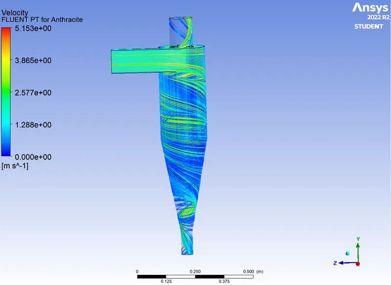
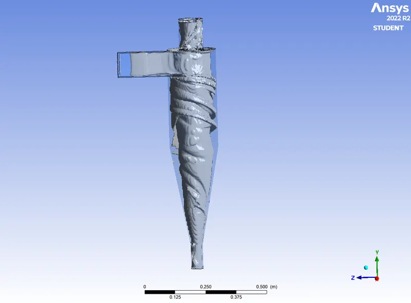
Case-iii    Diameter= 3e-6 at velocity = 3m/s

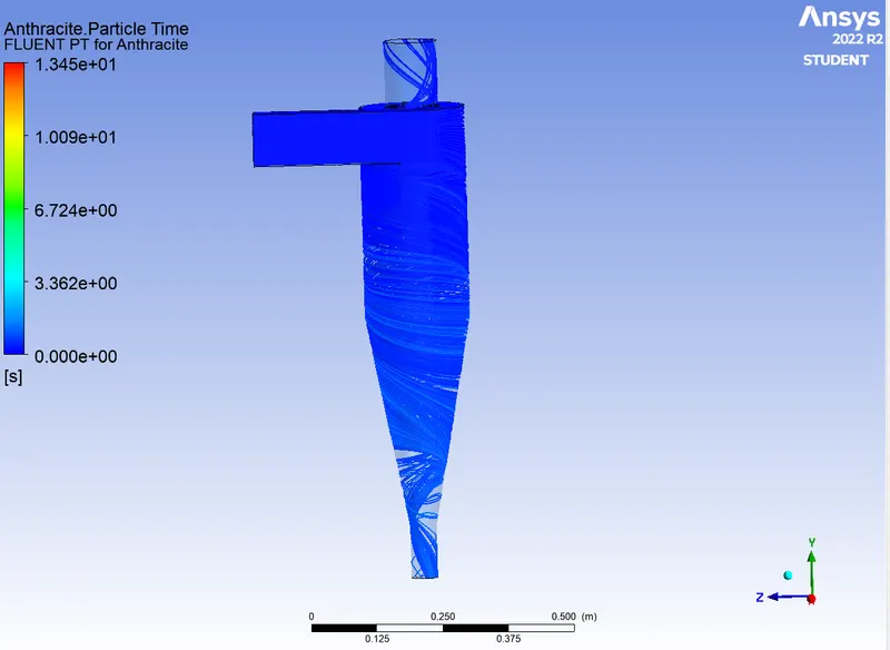
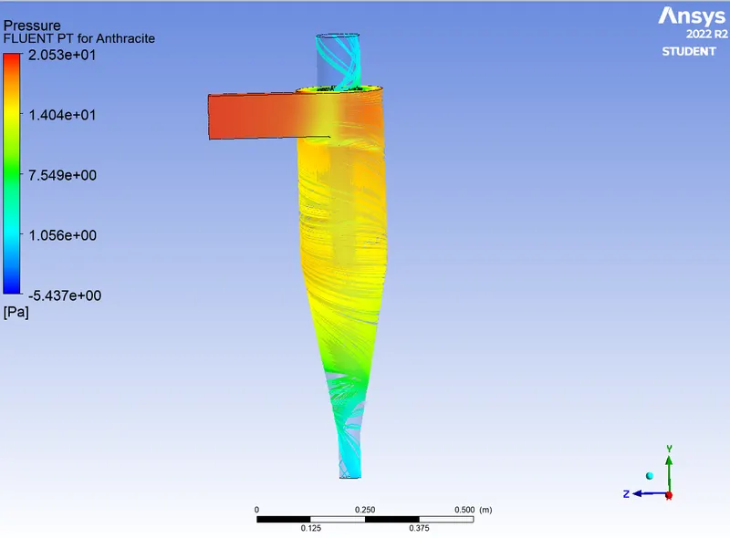
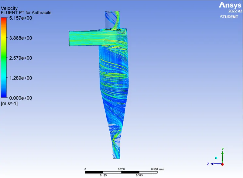
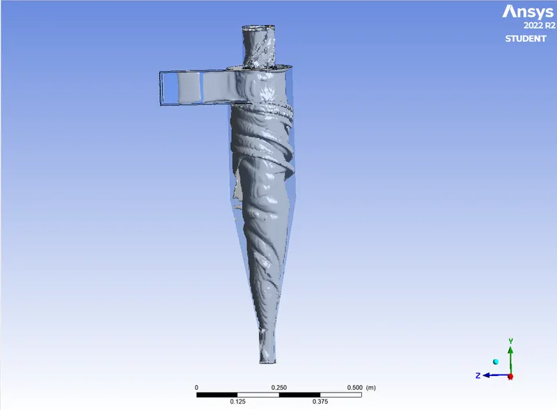
Case-iv    Diameter= 4e-6 at velocity = 3m/s

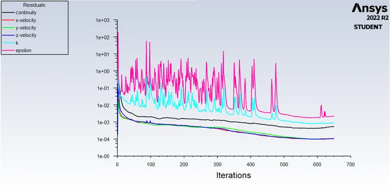
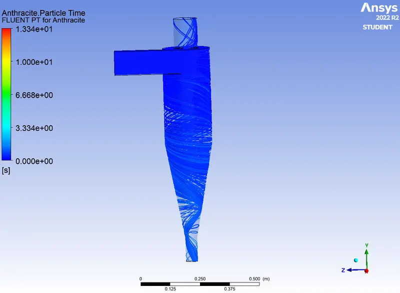
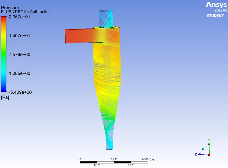
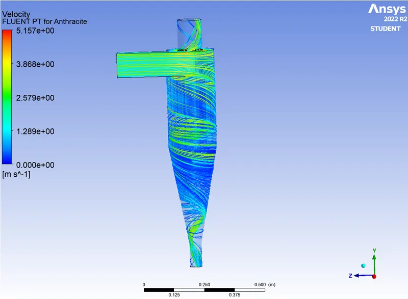
Case-v    Diameter= 5e-6 at velocity = 3m/s

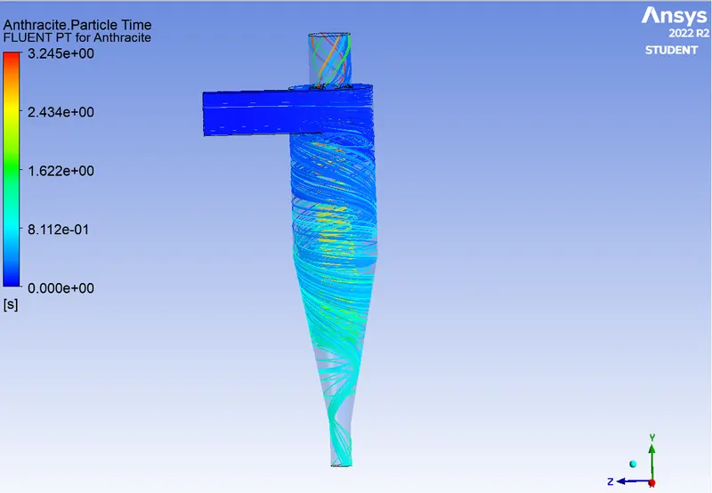
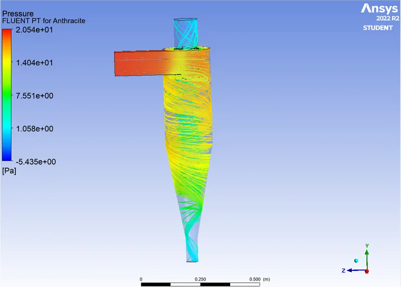
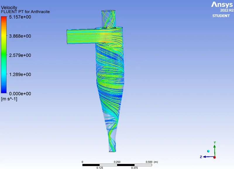
Calculation of separation efficiency of each case

Formula to calculate the separation efficiency of each case =

Seperation efficiency = (Particles Trapped/ Total Particles Tracked)* 100 

The below table gives the details of particle data obtained from the analysis and the separation efficiency calculated for each case.

Sl.no	Particle diameter(µm)	Particle tracked	Particle Trapped	Particles escaped	Incomplete	Seperation efficiency
1.	1e-6	378	331	47	-	87.5%
2.	2e-6	378	332	45	1	87.83%
3.	3e-6	378	334	43	1	88.35%
4.	4e-6	378	324	53	1	87.71%
5.	5e-6	378	292	86	-	77.24%

Part-2    To perform an analysis on a  given cyclone separator model by varying the particle velocity from 1 m/sec to 5 m/sec and calculate the separation efficiency and pressure drop in each case. Discuss the results. [Use particle diameter size as 5 μm for all cases & keep flow velocity same as particle velocity]

Case-i    Diameter= 5e-6 at velocity = 1m/s

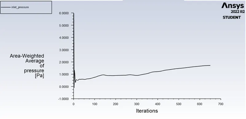
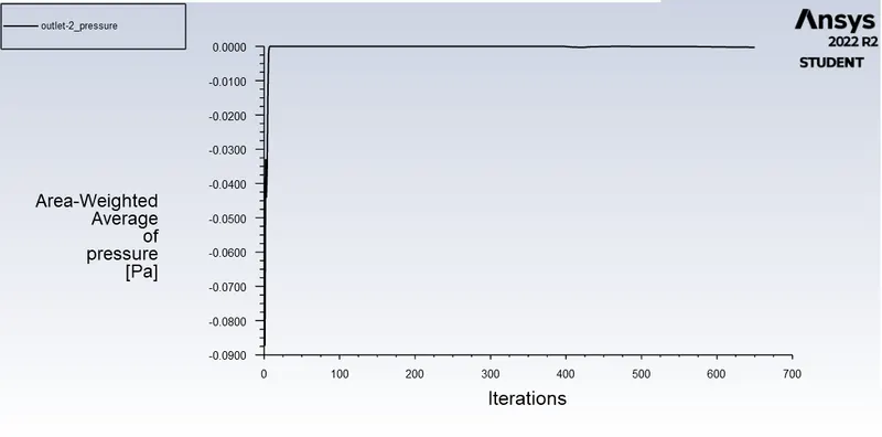
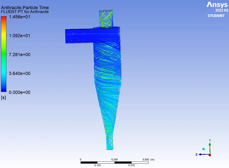
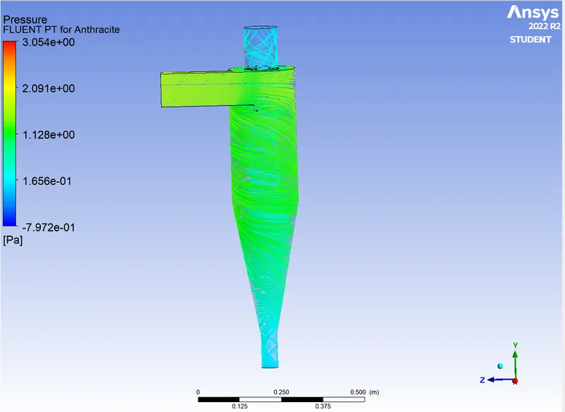
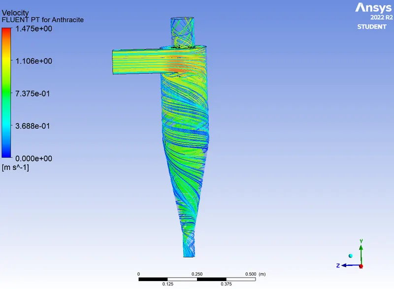
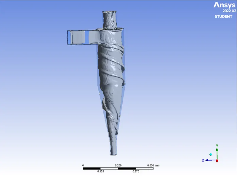
Case-ii    Diameter= 5e-6 at velocity = 2m/s

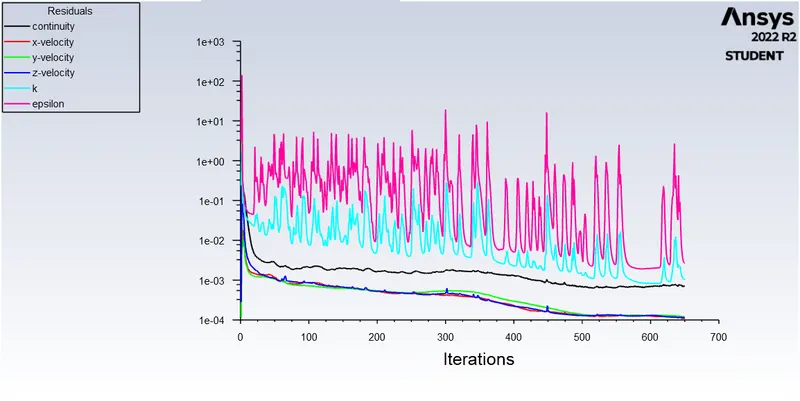
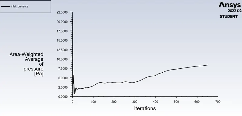
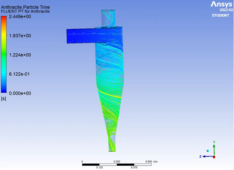
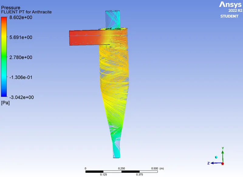
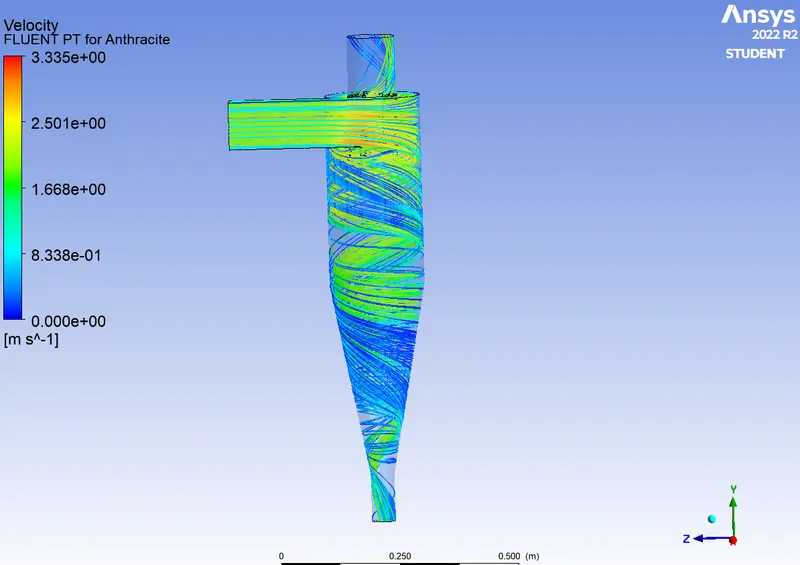
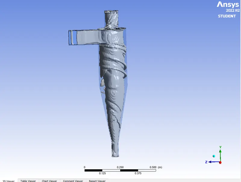
Case-iii    Diameter= 5e-6 at velocity = 3m/s

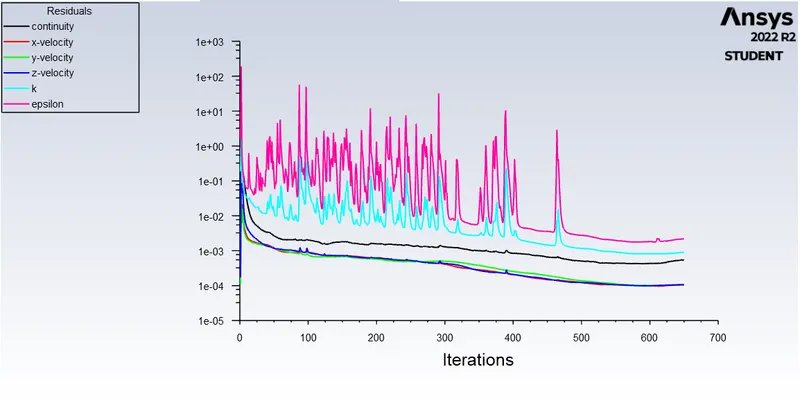
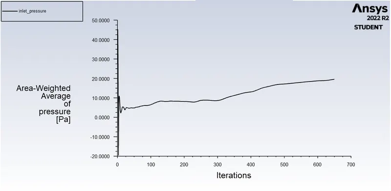
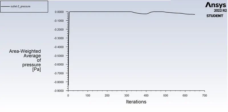
Case-iv    Diameter= 5e-6 at velocity = 4m/s

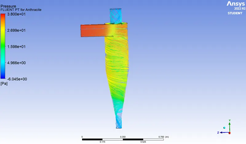
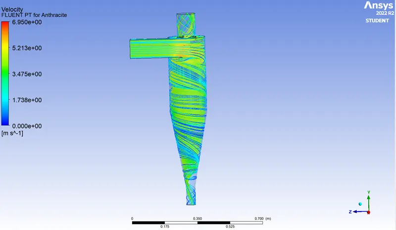
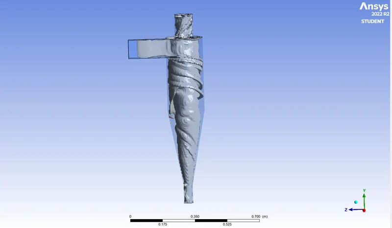
Case-v    Diameter= 5e-6 at velocity = 5m/s

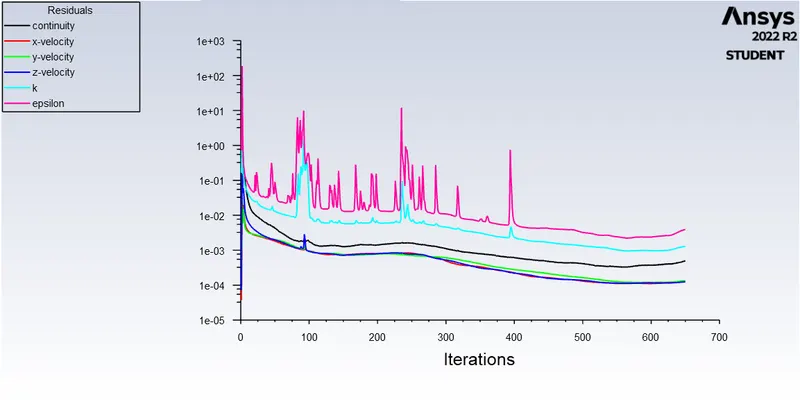
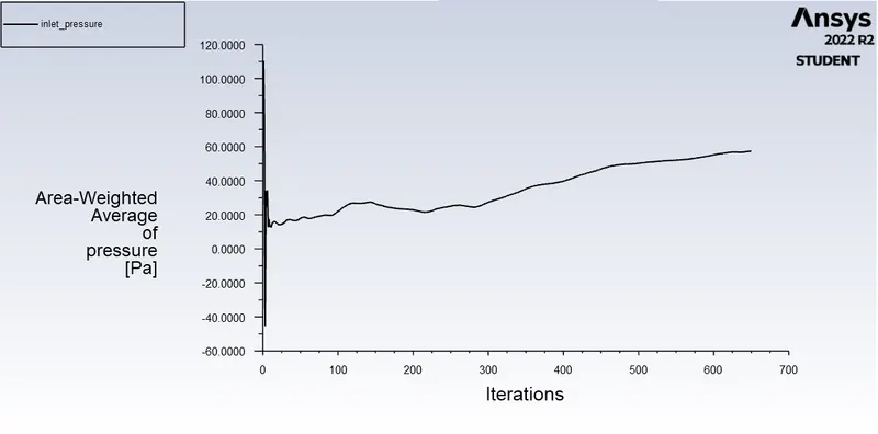
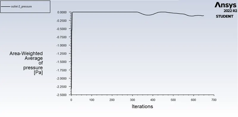
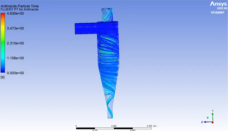
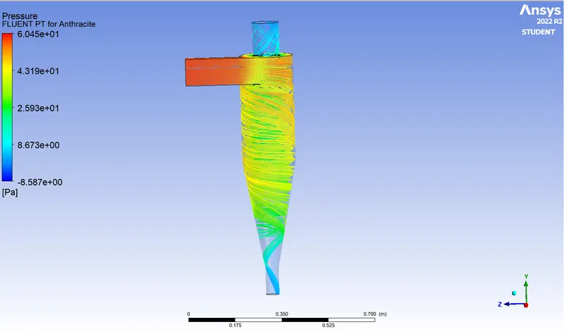
Calculation of separation efficiency of each case

Formula to calculate the separation efficiency of each case =

Separation efficiency = (Particles Trapped/ Total Particles Tracked)* 100 

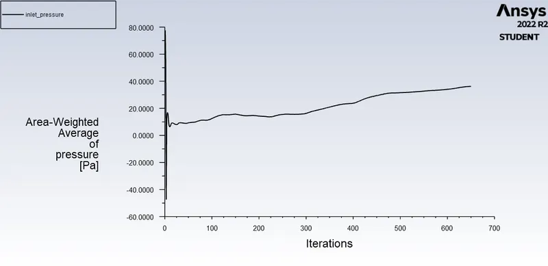
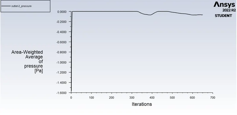
Pressure Drop = Pressure drop at the inlet - Pressure drop at the outlet

 The below table gives the details of particle data obtained from the analysis and the separation efficiency calculated for each case.

Sl.no	Flow velocity(m/s)	Pressure inlet (Pascal)	Pressure Outlet(Pascal)	Pressure Drop	Particle tracked	Particle Trapped	Particles escaped	Incomplete	Seperation efficiency
1.	1	1.716	-0.00028	1.716	378	277	100	1	73.2%
2.	2	8.357	-0.0088	8.365	378	319	59	-	84.3%
3.	3	19.5785	-0.0317	19.610	378	292	86	-	77.2%
4.	4	36.1504	-0.0680	36.218	378	267	111	-	70.6%
5.	5	57.3803	-0.1077	57.488	378	257	121	-	67.9%

Conclusion-

1. In the analysis of Part 1, it is observed that the separation efficiency increases as the particle diameter decreases.
2. In the analysis of Part 2, it is observed that the pressure drop on the cyclone seperator increases with the increase in inlet velocity of the particle. 
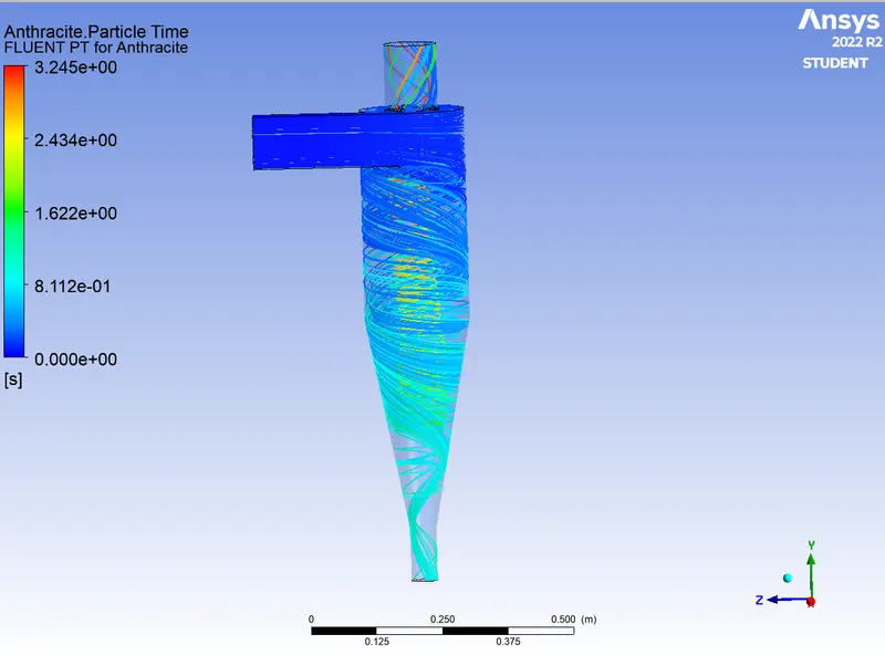
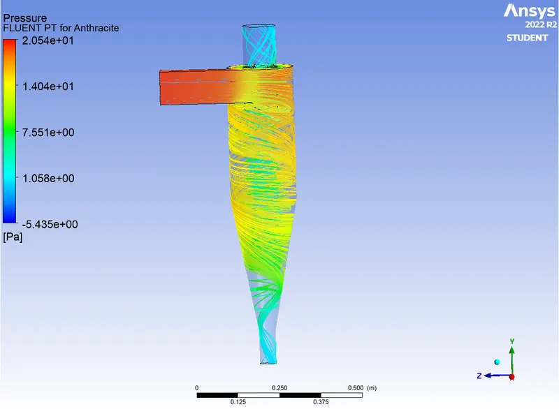
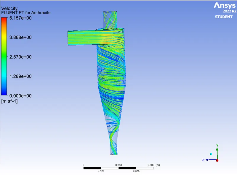
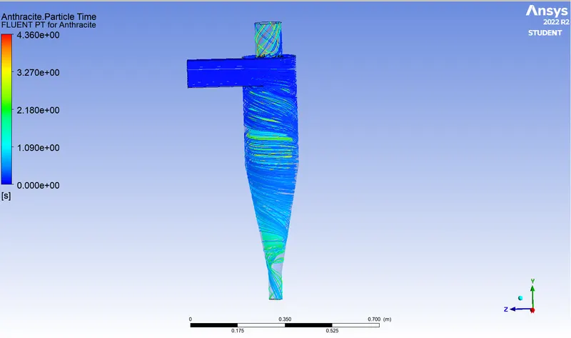
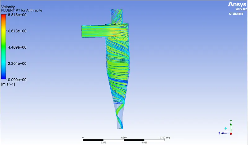
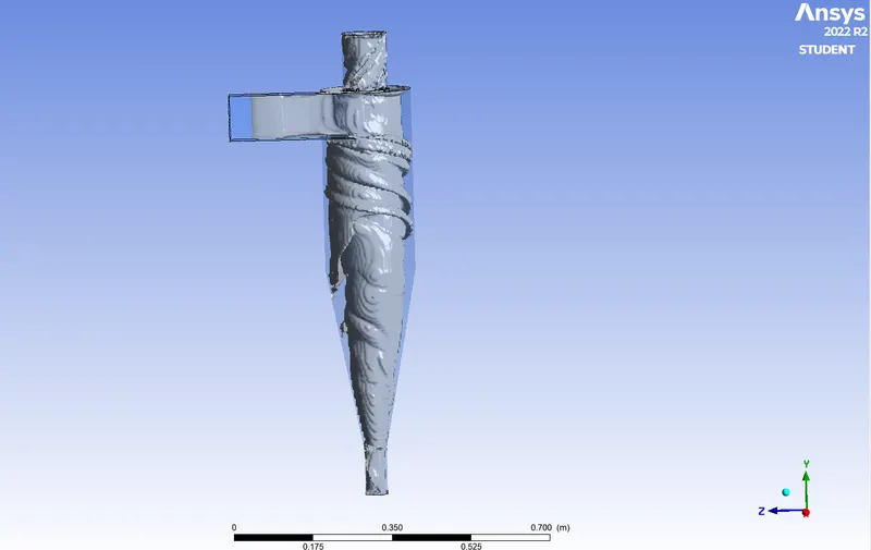
3. In both analysis, it is observed that the particles experience higher velocity near the barrel or middle cylinder part of the cyclone separator and hence the particles face high pressure near the barrel or middle cylinder part of the cyclone separator.