Week 8 - Simulating Cyclone separator with Discrete Phase Modelling

Objective: To perform analysis on cyclone separator and calculate the separation efficiency and pressure drop.

Introduction:

Experiments performed to study the physics of certain phenomenon are costly and time-consuming. Numerical simulation is developed and used to reduce the time needed to study the nature and physics involved in the system of interest. This method indeed provides results very fast compared to experiments but they lack a bit in terms of accuracy. If the experiments take a month to produce results, simulation might take a day and give us results 90% accurate. In the fast-paced world, where developing various solutions require faster results, engineers make a delicate balance between the accuracy and time taken as necessary.

All fluid flows are governed by three equations -Continuity, momentum and energy equations. We need to solve these equations for the given conditions to understand the fluid behavior. Computers are incapable of solving these equations in their integral and differential forms. So, we can divide our geometry into many tiny elements (called mesh) and modify the governing equations into difference equations that can be solved by the computer. We apply these difference equations for all the elements in the geometry and generate an approximate solution. It is hence necessary to validate these results against the experimental data.

The number of difference equations, for a given problem varies with the nature of physics involved. We typically solve a finite number of equations at all the elements. These equations are grouped together, called a turbulence model. A lot of work has been put into developing and improving the turbulence models and the work still goes on today. Examples of turbulence models are S-A, k-epsilon, k-omega etc.

Theory:

Cyclone Separator:

Cyclone separators are separation devices that use the principle of inertia to remove particulate matter from flue gases. A cyclone separator is one of many air pollution control devices known as pre-cleaners since they generally remove larger pieces of particulate matter. This prevents finer filtration methods from having to deal with large, more abrasive particles later on. In addition, several cyclone separators can operate in parallel, and this system is known as a multi-cyclone.

Four empirical models that can calculate the efficiency of a cyclone separator.

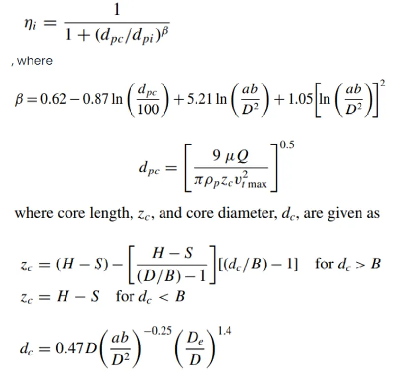
Iozia and Leith model:

This model was developed based on force balance. In this model, since the particle undergoes vortex flow, two main forces are considered, centrifugal force and flow resistance. The collection efficiency(η_i) of particle diameter(d_pi) is given as

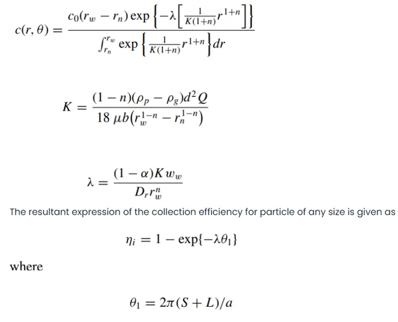
Li and Wang model:

This model includes particle bounce or re-entrainment and turbulent diffusion at the cyclone wall. In this model, 2D analytical expression of particle distribution in the cyclone is given as

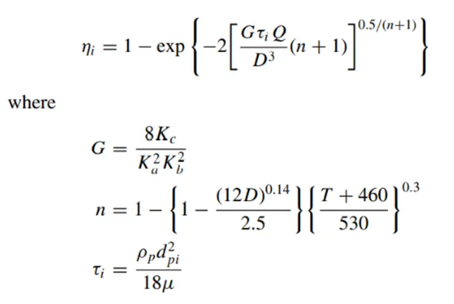
Koch and Licht model:

This model includes the inherently turbulent nature of cyclones and the distribution of gas residence times within the cyclone. A force balance and an equation on the particles collection yields the grade efficiency (η_i) as

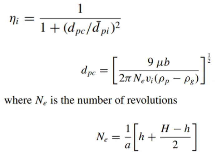
Lapple model:

This model was developed based on force balance without considering the flow resistance. Lapple assumed that a particle entering the cyclone is evenly distributed across the inlet opening. The efficiency of collection of any size of particle is given as

Modelling in Ansys Fluent:

The work flow in Ansys Fluent would follow four steps:

1. Geometry creation.
2. Mesh generation.
3. Pre-processing settings and simulation.
4. Extracting results.

Geometry creation:

We drag and drop the Fluent module to create the standalone system. We open the geometry editing section- space claim and import the given model. We can close space claim and the model is saved automatically.

Mesh generation:

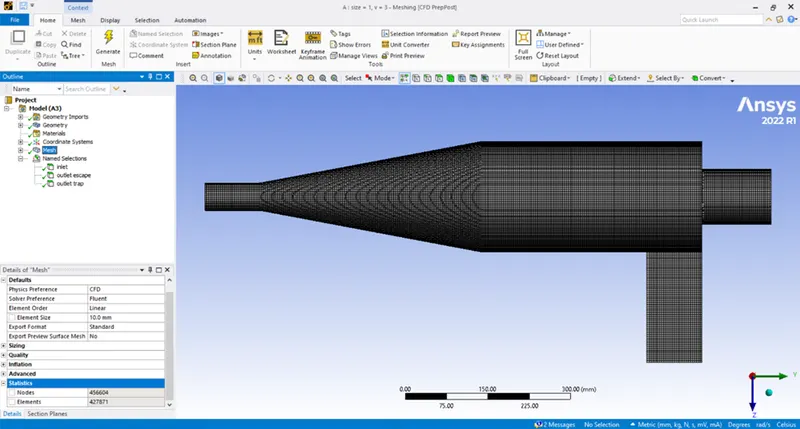
We use a default cartesian mesh of 10mm with 4,27,871 elements. We assign appropriate named selections to make it easier to work in the simulation section later. Here, we assigned inlet, outlet escape and outlet trap. We close the window and the changes are updated in the system.

Pre-processing settings and Simulation:

We would proceed to Setup the conditions of the model. The process flow would be as follows:

1. Check the mesh in the solver.
2. Choose the turbulence model.
3. Enable discrete-phase model.
4. Run the simulation for given number of time steps.

Extracting results:

We open the results section where we can use various visualizing tools like transparency and colouring the created surfaces with the instantaneous variables like temperature, velocity and obtain contours, charts and plots. We need to run the simulation until the residual values are either reach the convergence criteria or display a periodic pattern.

Settings used for current simulation:

We used Pressure-based solver, absolute velocity formulation, steady state simulation.

We enabled gravity and used RNG k-epsilon model with swirl dominated flow. We use air as the working media.

We would enable discrete-phase model and input the particle size and velocity at which the particles enter the model as shown. It should be noted that the number of particles in the given simulation is equal to the number of mesh elements in the inlet surface.

The particle material used for the simulation is anthracite.

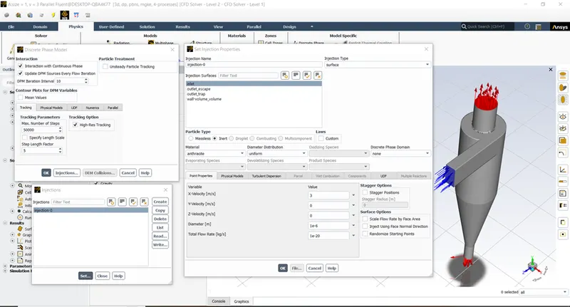
We will study the efficiency of the cyclone separator using both size of the particles and velocity of particle injection as parameters. The cases would look like this.

Cases	Size of particle (µm)	Velocity (m/s)
1	1	3
2	3	3
3	5	3
4	5	1
5	5	3

Based on the mesh at inlet, there are 378 particles that are being tracked, the cyclone separator is expected to trap most of these particles and thus have filtered the air.

Case 1- size- 1µm and velocity- 3m/s:

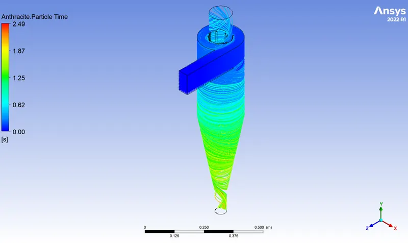
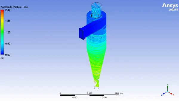
Anthracite particle time:

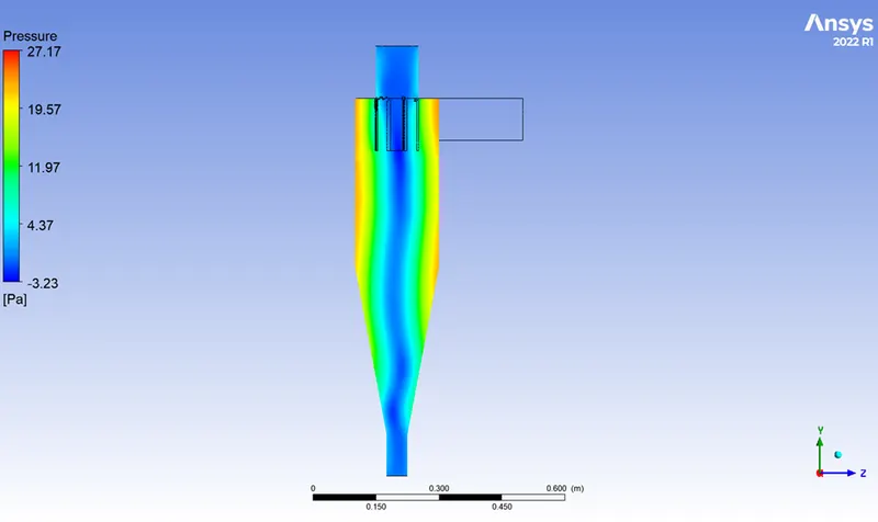
Pressure contour:

Velocity contour:

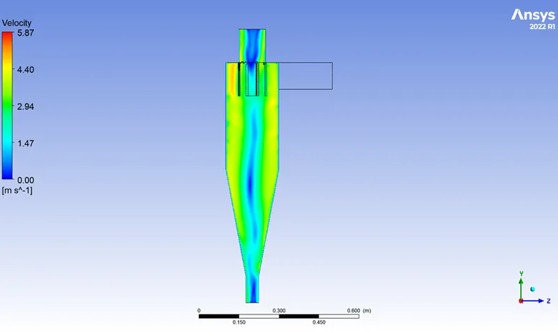
Animation:

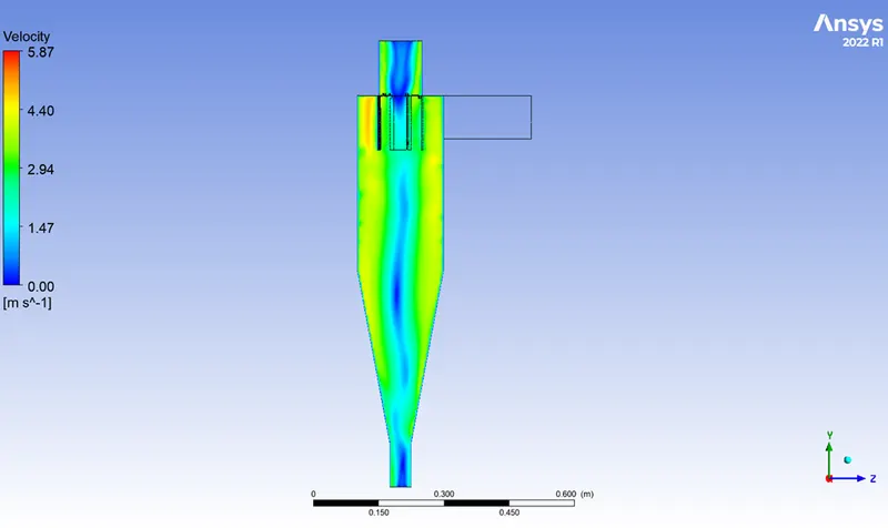
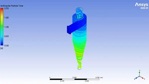
Case 2- size- 3µm and velocity- 3m/s:

Anthracite particle time:

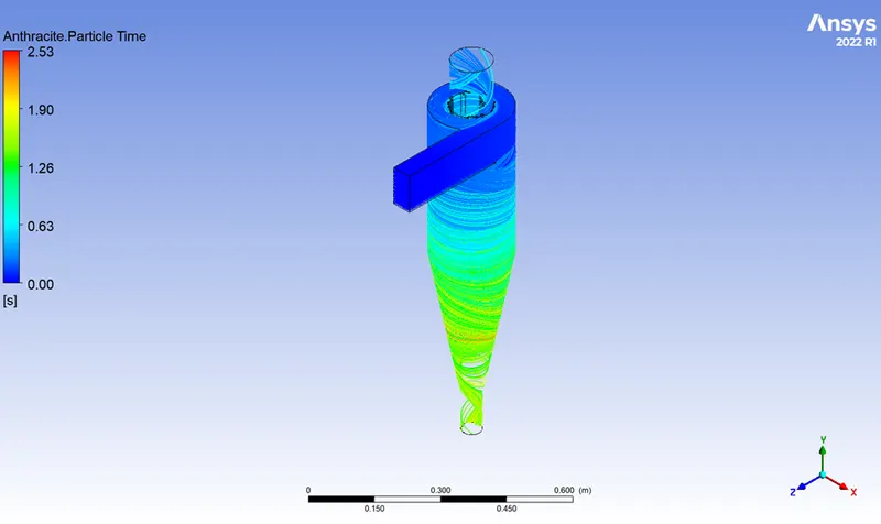
Pressure contour:

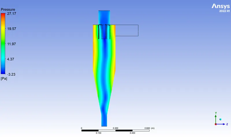
Velocity contour:

Animation:

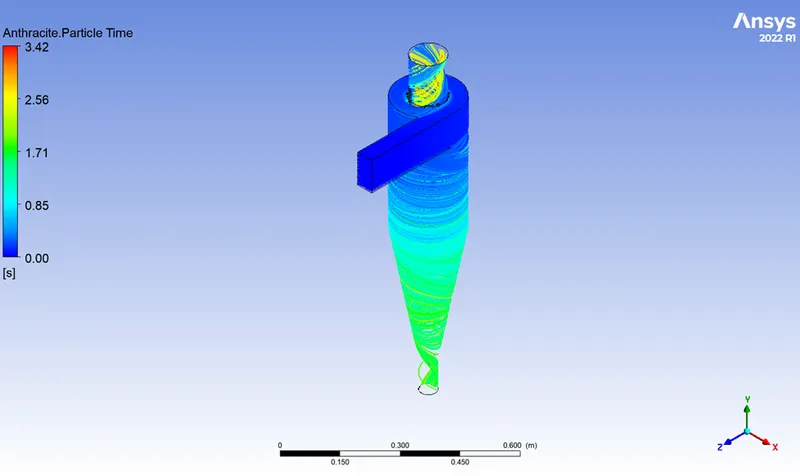
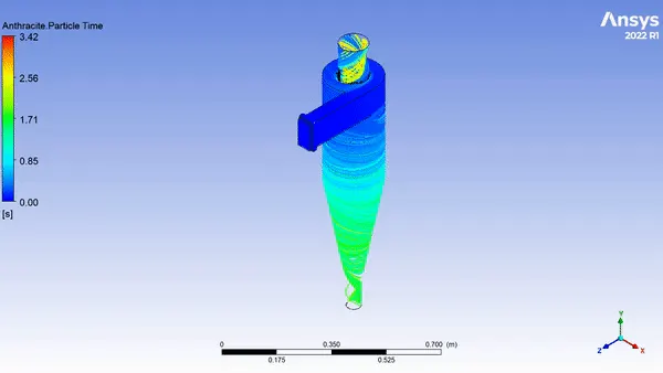
Case 3- size- 5µm and velocity- 3m/s:

Anthracite particle time:

Pressure contour:

Velocity contour:

Animation:

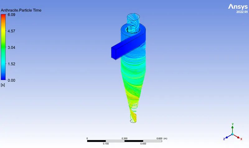
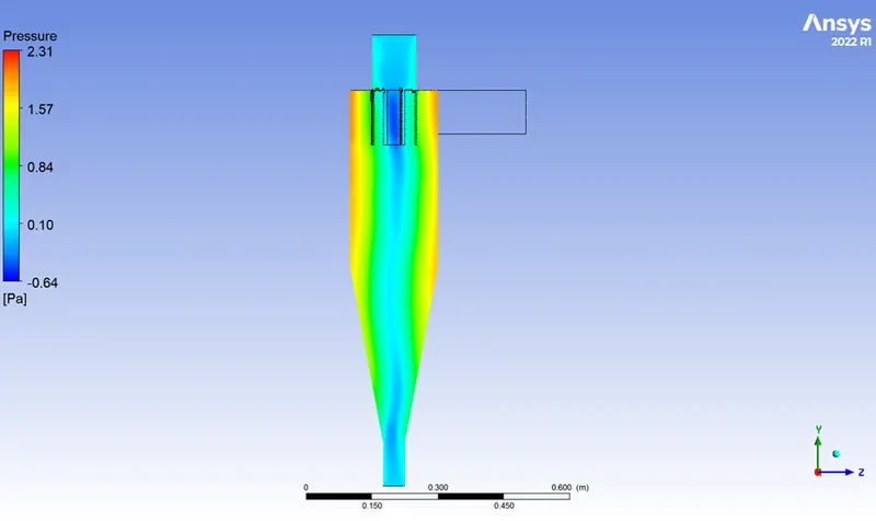
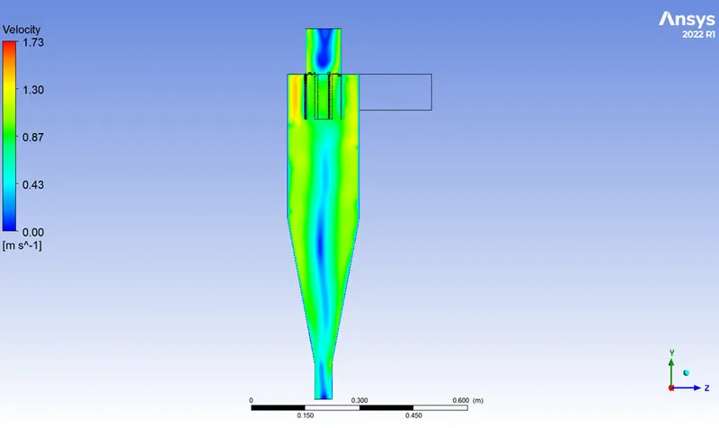
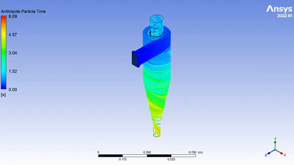
Case 4- size- 5µm and velocity- 1m/s:

Anthracite particle time:

Pressure contour:

Velocity contour:

Animation:

Case 5- size- 5µm and velocity- 5m/s:

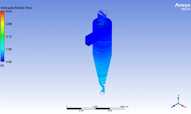
Anthracite particle time:

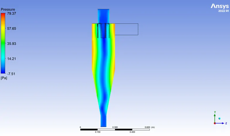
Pressure contour:

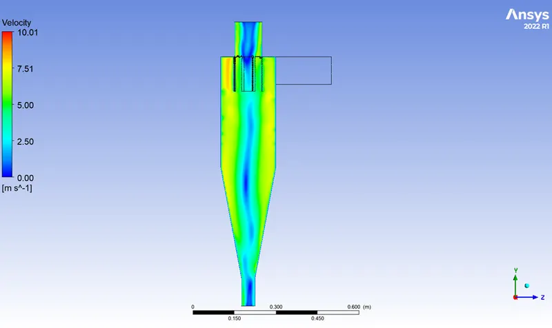
Velocity contour:

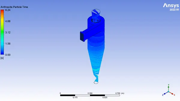
Animation:

The details of pressure drop and cyclone efficiency are tabulated.

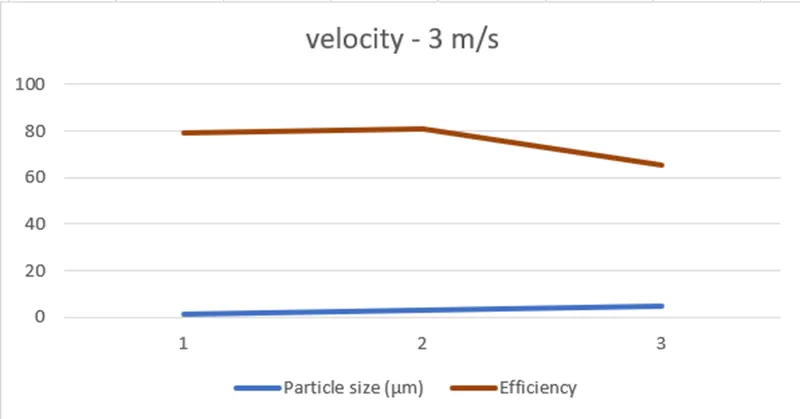
We have fixed velocity as 3 m/s. We see that the efficiency is almost constant for particle sizes 1 and 3µm and reduces for 5µm. This can be because of the interaction between the particles.

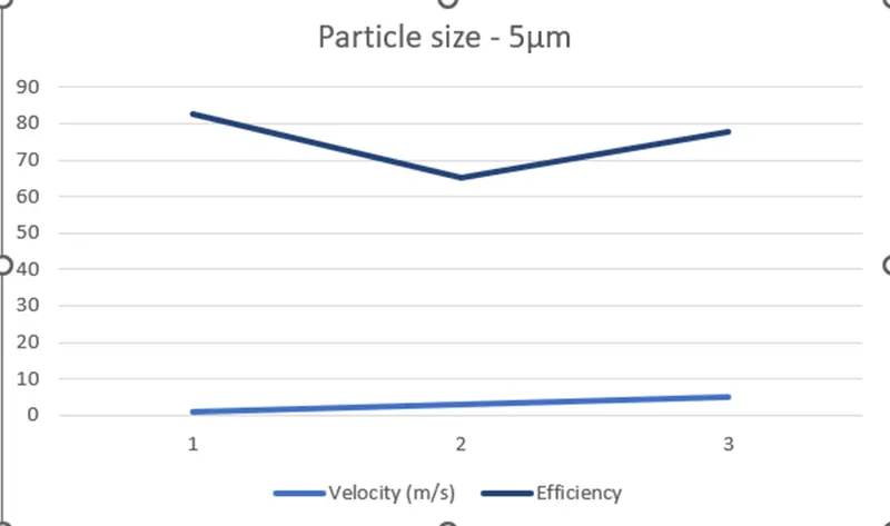
We have fixed the particle size as 5 µm. We see that the efficiency reduces and then increases. This can be because of the interaction between the particles.

Conclusion:

The expected trend was with increase in velocity and particle size the cyclone separator efficiency increases. The deviation from the trend can be attributed to the interaction between the particles due to a large number of them.

References:

1. Wang, D.L. Xu, K.W. Chu, A.B. Yu, Numerical study of gas–solid flow in a cyclone separator, Applied Mathematical Modelling, Volume 30, Issue 11, 2006, Pages 1326-1342, ISSN 0307-904X.
2. Gimbun, Jolius & Luqman Chuah, Abdullah & Choong, TSY & Fakhru'l-Razi, A. (2005), A CFD Study on the Prediction of Cyclone Collection Efficiency, International Journal for Computational Methods in Engineering Science and Mechanics, Vol 6. 161-168.