Week 8 - Simulating Cyclone separator with Discrete Phase Modelling

Simulating Cyclone separator with Discrete Phase Modelling

AIM:

To perform analysis on cyclone separator and calculate the separation efficiency and pressure drop.

OBJECTIVES:

1. Write a few words about any four empirical models used to calculate the cyclone separator efficiency.
2. To perform an analysis on a given cyclone separator model by varying the particle diameter from 1 μm to 5 μm and calculate the separation efficiency in each case. Discuss the results. [Use both the velocity's as 3 m/sec.]
3. To perform an analysis on a given cyclone separator model by varying the particle velocity from 1 m/sec to 5 m/sec and to calculate the separation efficiency and pressure drop in each case. Discuss the results. [Use particle diameter size as 5 μm for all cases & keep flow velocity same as particle velocity).

THEORY:

CYCLONE EFFICIENCY EMPIRICAL MODELS

1. Iozia and Leith Model

Iozia and Leith logistic model is coined based on force balance. This model is a modification of the Barth Model. This model assumes that a particle carried by the vortex endures the influence of two forces: a centrifugal force and flow resistance. The collection efficiency η_i of particle diameter d_pi can be calculated from

β is an expression for slope parameter derived based on the statistical analysis of experimental data of a cyclone with D = 0.25 m and d_pc is the 50% cut size.

2. Koch and Licht Model

The collection theory by Koch and Licht studied the inherently turbulent nature of cyclones and the distribution of gas residence times within the cyclone. The following assumptions were made by Koch and Licht while describing the particle motion in the entry and collection regions.

• The tangential velocity of a particle is equal to the tangential velocity of the gas flow, i.e. there is no slip in the tangential direction between the particle and the gas.
• The tangential velocity is related to the radius of the cyclone

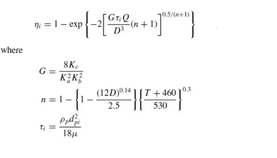
A force balance and an equation on the particles collection yield the grade efficiency η_i

3. Li and Wang Model

Particle bounce or re-entrainment and turbulent diffusion at the cyclone wall are included in the Li and Wang model. A two-dimensional analytical expression of particle distribution in the cyclone is obtained. The following assumptions were made while proposing this model,

• The radial particle velocity and the radial concentration profile are not constant for uncollected particles within the cyclone.
• Boundary conditions with the consideration of turbulent diffusion coefficient and particle bounce re-entrainment on the cyclone wall are:

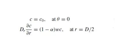
• The tangential velocity is related to the radius of the cyclone.

The concentration distribution in a cyclone is given as:

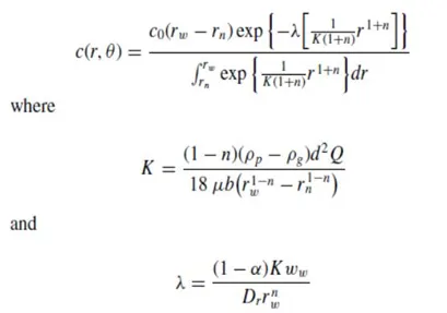
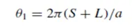
The resultant expression of the collection efficiency for particles of any size is given as

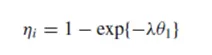
where

4. Lapple Model

Force balance without considering the flow resistance is the basis of the Lapple model. Lapple assumed that a particle entering the cyclone is evenly distributed across the inlet opening. The particle that travels from the inlet half-width to the wall in the cyclone is collected with 50% efficiency.

The efficiency of collection of any size of the particle is given by

MODELLING APPROACH :

• Import and extract fluid volume from the 3D model of the cyclone separator.
• Provide Body Cartesian sizing for a structured mesh,
• The viscous model is set as K-epsilon RNG with 'swirl dominated flow' and standard wall treatment.
• Enable Discrete Phase Modeling(DPM) with coupled interaction between the phases.
• The material of injection is selected as Anthracite.
• Boundary conditions are set as

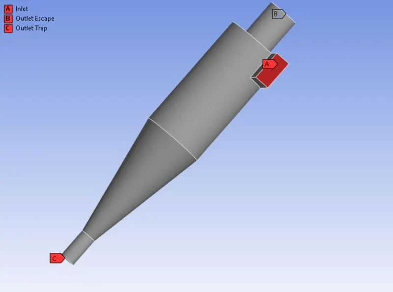
1. Inlet and Wall - Reflect
2. Outlet(top) - Escape
3. Outlet(bottom) - Trap

• Use Standard initialization and select compute from the inlet.

PREPROCESSING :

Geometry

• Import the 3D geometry of the cyclone separator to Spaceclaim.

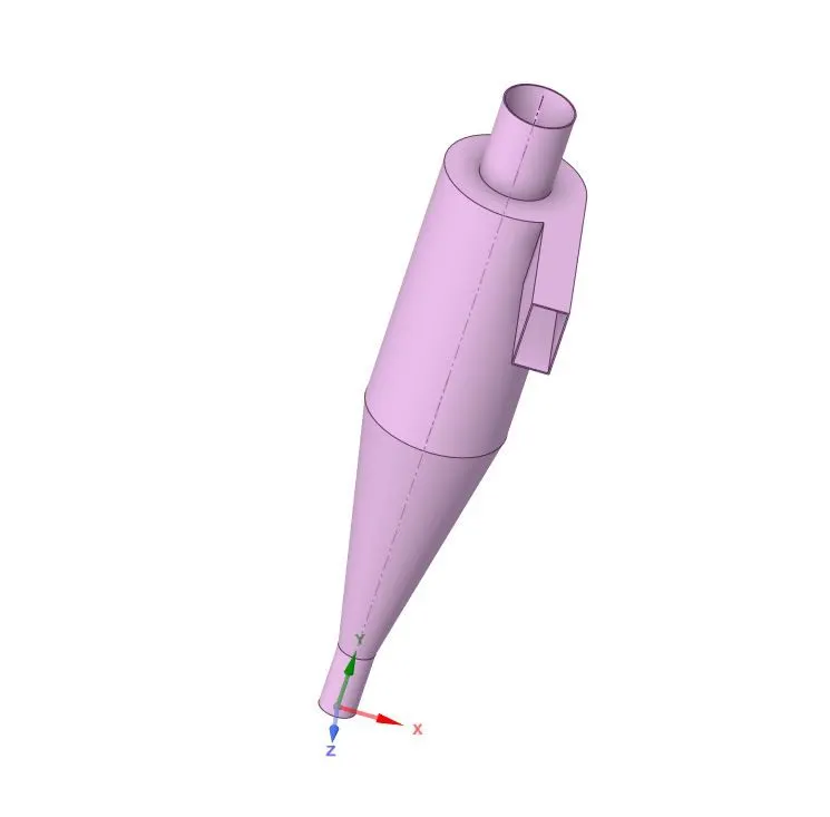
• Now using the Volume Extract tool, extract the fluid volume.

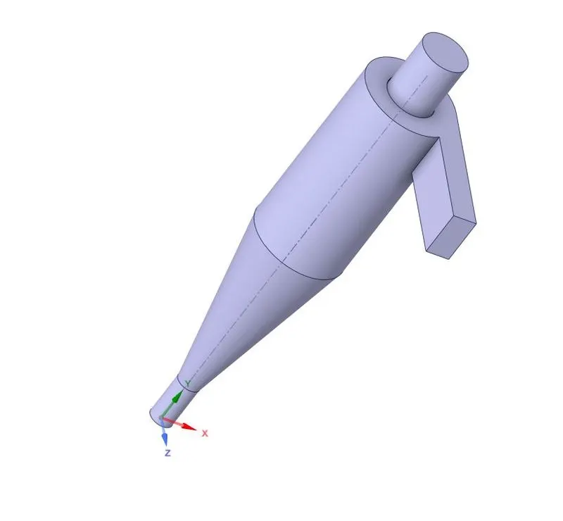
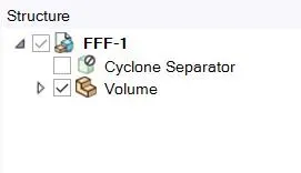
• Untick the cyclone separator and use the 'suppress for physics' option so that the solid material won't interfere with the simulation.

Meshing :

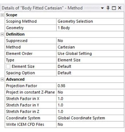
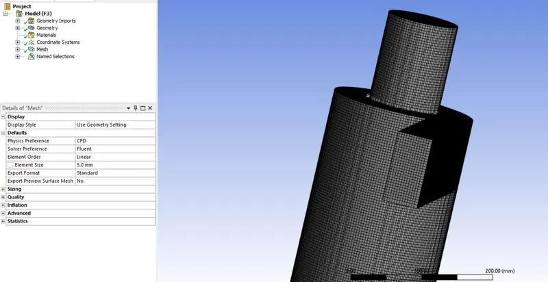
• Generate mesh with an element size of 5mm.
• Use the 'Body Fitted Cartesian' for a structured mesh.

• Give appropriate 'Named selections' as per the problem statement.

• Update the mesh and exit.

Solver Setup

1.	Solver Type	Pressure Based
2.	Solver Time	Steady State
3.	Gravity	Enabled
4.	Viscous Model	K epsilon
5.	DPM	Enabled
6.	Injection (Anthracite)	Surface Injection
7.	Particle Diameter	1 to 5 micrometers
8.	Particle Velocity	1 to 5 m/s
9.	Material	Air
10.	Inlet	Velocity Inlet DPM - Reflect
11.	Outlet 1 (Top)	DPM - Escape
12.	Outlet 2 (Bottom)	DPM - Trap

• Gravity is set as -9.81m/s in the y-direction.
• The RNG K-epsilon model with swirl dominant flow and standard wall treatment is selected as the viscous model.
• Second Order Upwind scheme is selected for both the Turbulent dissipation rate and Turbulent kinetic energy.
• The solution method is selected as SIMPLE.
• After performing Standard Initialization, run the simulation for 600 iterations.

RESULTS :

Analysis by varying particle diameter (velocity - 3 m/s)

1 μm

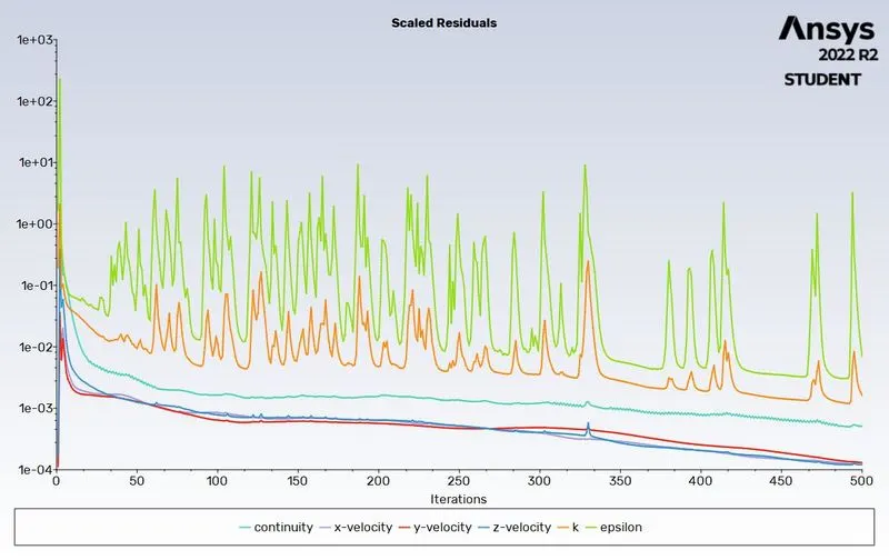
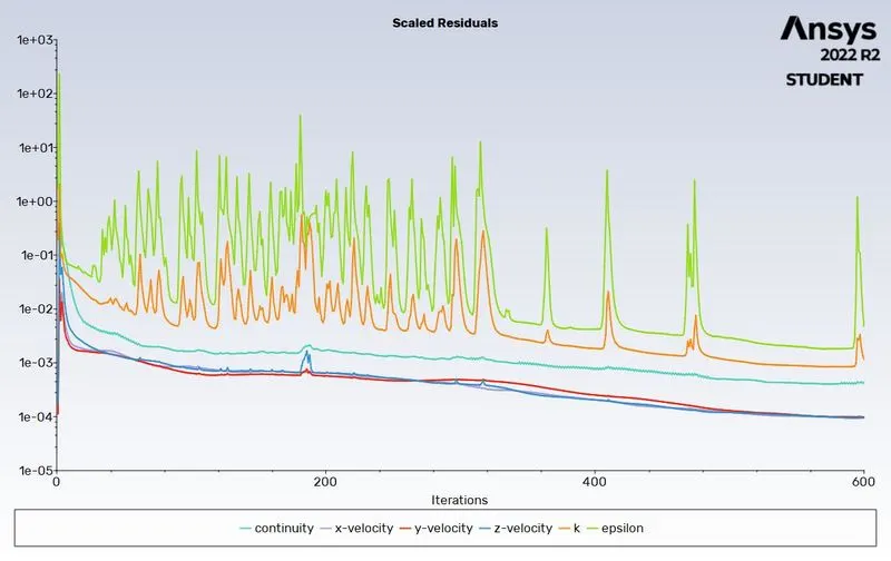
• Residuals

• DPM iteration

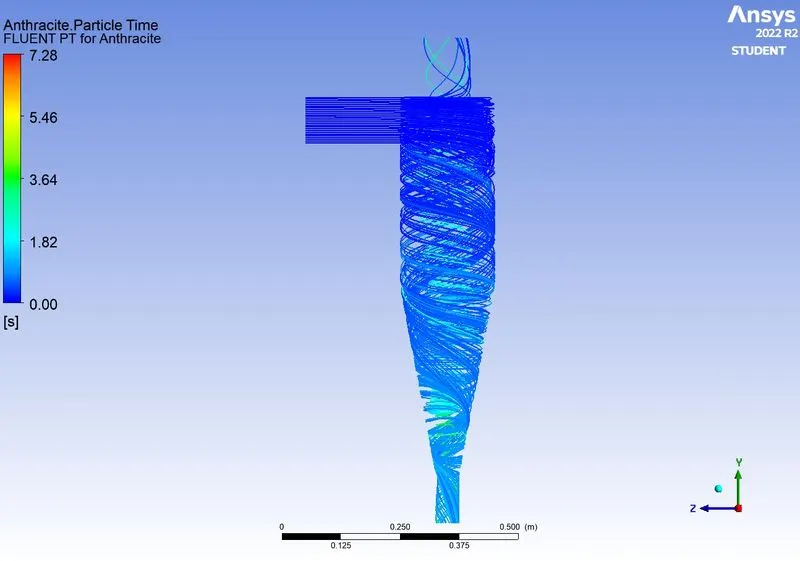
• Anthracite Particle Time

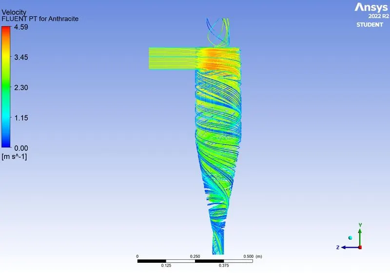
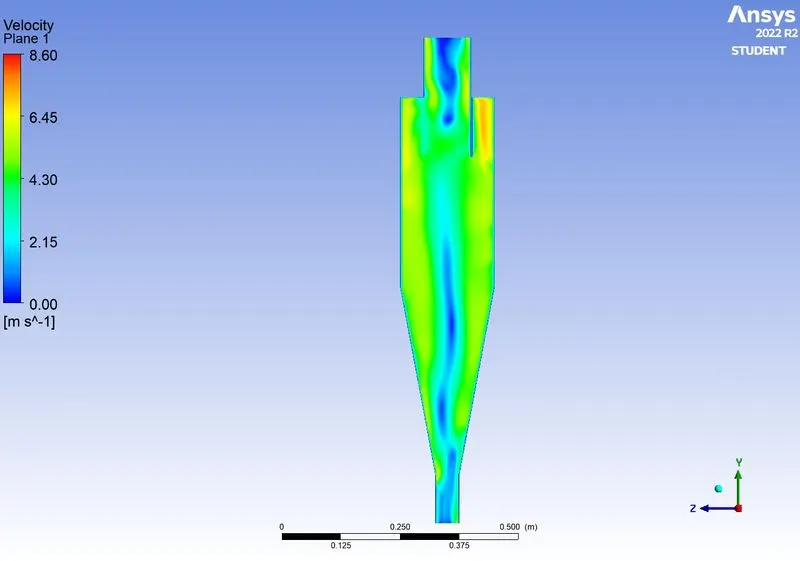
• Velocity contour

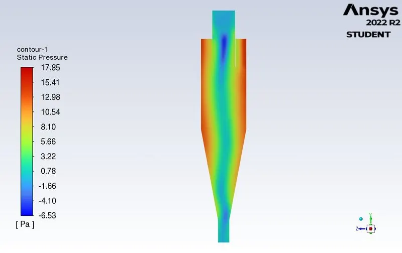
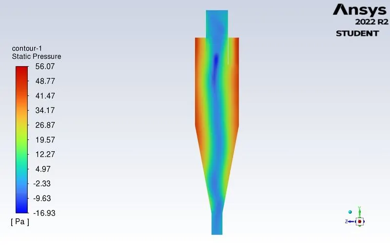
• Pressure contour

μm

• Residuals

• DPM iteration

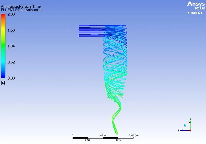
• Anthracite Particle Time

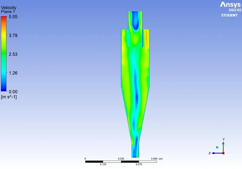
• Velocity contour

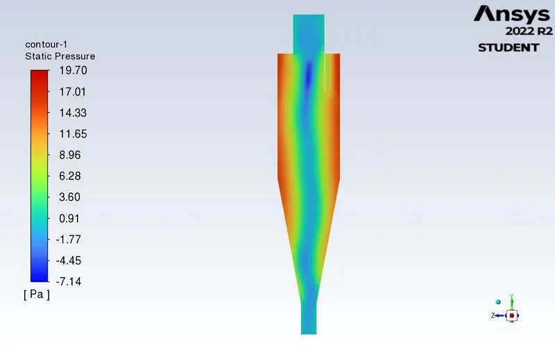
• Pressure contour

5 μm

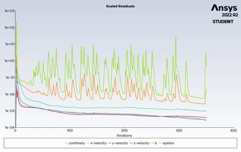
• Residuals

• DPM iteration

• Anthracite Particle Time

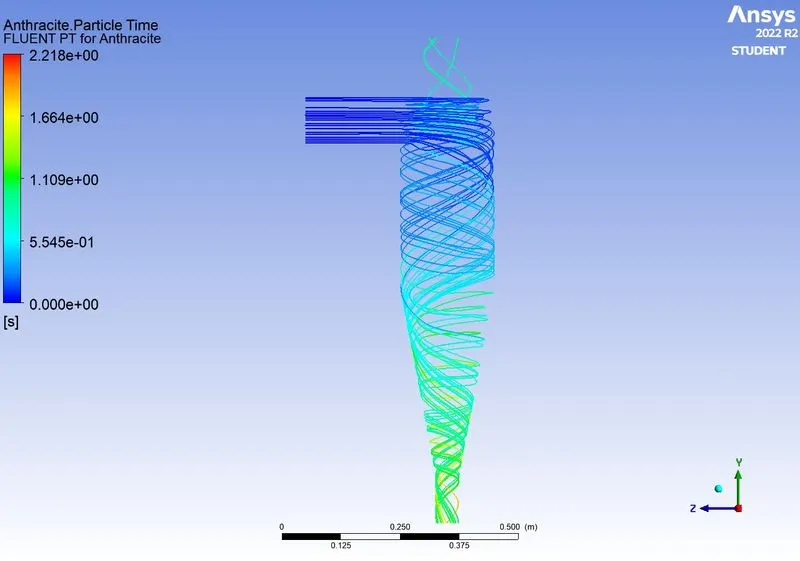
• Velocity contour

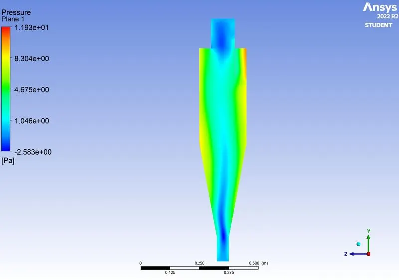
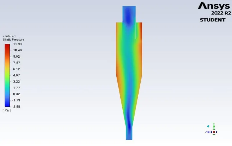
• Pressure contour

Analysis by varying particle velocity (particle size - 5 μm)

1 m/s

• Residuals

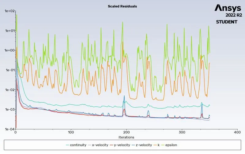
• DPM iteration

• Anthracite Particle Time

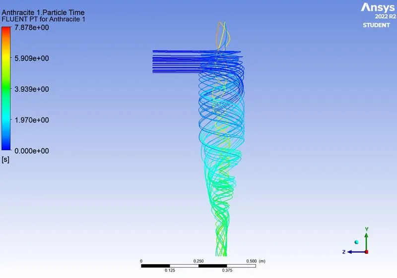
• Velocity contour

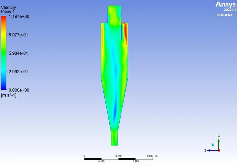
5 m/s

• Residuals

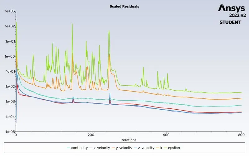
• DPM iteration

• Anthracite Particle Time

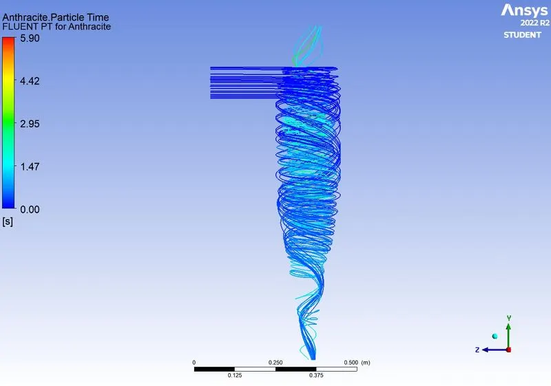
• Velocity contour

• Pressure contour

Sweep Animation

• Particle velocity of 3 m/s

1 μm - https://drive.google.com/file/d/1b4XwcXmxhUk5d54_vUy8aaLcE-pMgopp/view?usp=sharing

3 μm - https://drive.google.com/file/d/1RtIbNx6yNOLjPqbG2WeK5ksg-TTbku9s/view?usp=sharing

5 μm - https://drive.google.com/file/d/1bE1Yz6fzN_1Xhit6ljAHZ06DrXR6lKrk/view?usp=sharing

• Particle diameter of 5 μm

1 m/s - https://drive.google.com/file/d/17B4VWnpt89MYUDvupNxbwIYhIS2G6qKa/view?usp=sharing

5 m/s - https://drive.google.com/file/d/1IoQDS6WkTvu-TO5P5i8PJ6LIVLAUf4x5/view?usp=sharing

Cyclone Separator Efficiency

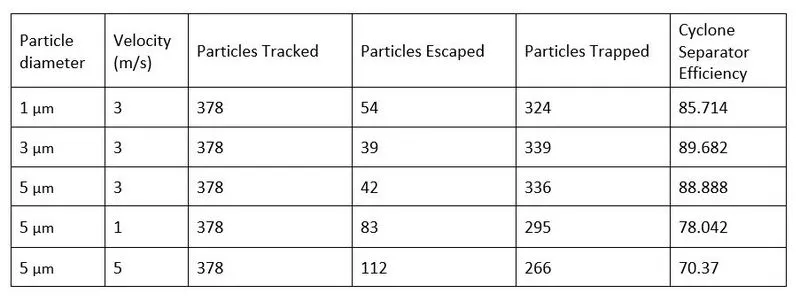
• Comparison Table

CONCLUSIONS :

• Simulation is done for particle size varying from 1μm to 5μm with air and particle velocity as 3m/s.
• The efficiency of the cyclone separator decreases with a decrease in particle diameter.
• Higher velocities yield higher efficiency. But in this simulation, we can observe that for a particle size of 5 micrometers and particle velocity of 5 m/s, the efficiency is actually low. This might be due to an increase in pressure drop.

REFERENCES :

• https://www.researchgate.net/publication/232747389_A_CFD_Study_on_the_Prediction_of_Cyclone_Collection_Efficiency