Week 8 - Simulating Cyclone separator with Discrete Phase Modelling

The aim of this exercise is to simulate cyclone separator with discrete phase modelling (DPM). For this, there are 4 types of empirical models used to calculate the cyclone separator's efficiency. These are as follows:

1) Li and wang model: This model includes bounce and turbulent diffusion of a particle on the wall. From this, a 2D representation of the distribution of the particle can be obtained.

2) Lozia and Leith model: This model is based on the force balance and is based on the concept that a particle which is carried away by the vortex generated is under the influence of two different forces namely centrifugal force and flow resistance.

3) Lapple model: This model does not consider the flow resistance. instead, it is based on the force balance and inside the cyclone separator, the particles are evenly distributed across the inlet.

4)Koch and Licht model: This model assumes that for a particle, the tangential velocity is equal to that of a gas flow. This model also is based upon the concept of the turbulent nature of cyclones and distribution of the gas residence times inside the separator.

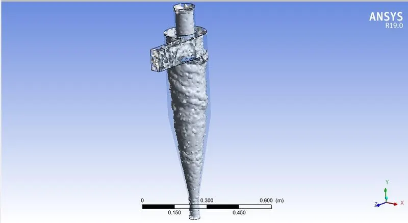
Now, for the simulation, first we obtain the model for a cyclone separator and import the model into spaceclaim. Now, we extract the volume of the cyclone separator using volume extract option under prepare and then save the file. Now we update the geometry and enter meshing. Inside meshing, we create named selections for the inlet, outlet 1 and outlet 2 and then generate mesh. The mesh size is specified as 10mm.

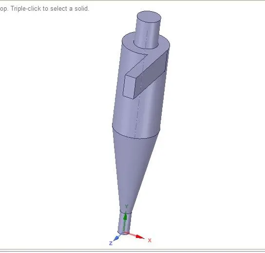
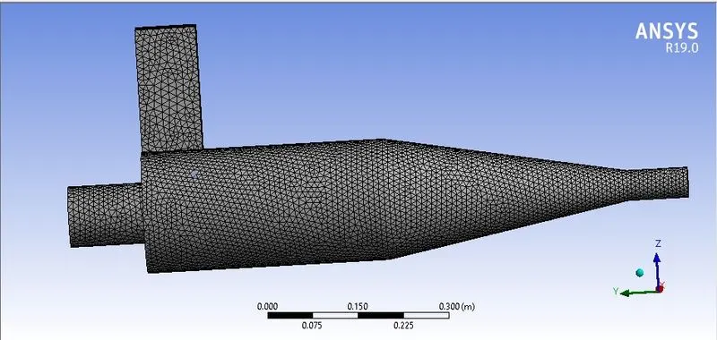
Now we enter fluent setup where we specify all the necessary parameters materials and boundary conditions fot the simulation to run. First, we choose steady state pressure baseed absolute velocity formation solver from setting up physics and enable gravity for negative y direction. We choose the k epsilon viscous model with RNG and swirl dominated flow. Now, under discrete phase, we choose interaction with continuous phase and update dpm every flow iteration and under injections, we create new and specify the velocity of the particle, material as anthracite as well as the particle diameter.

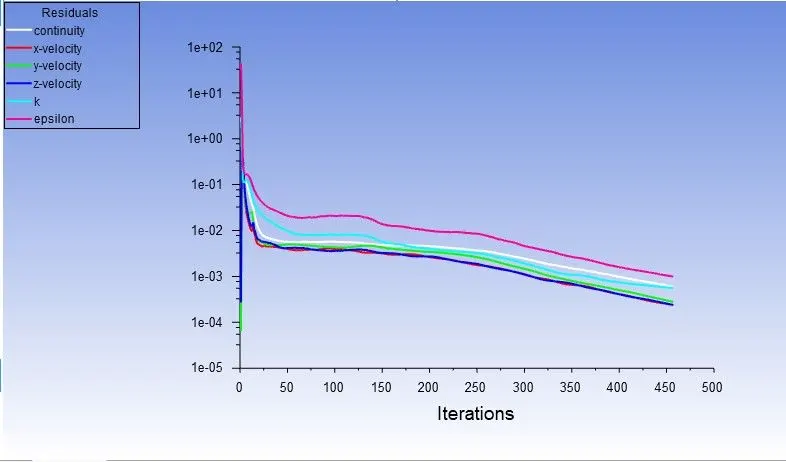
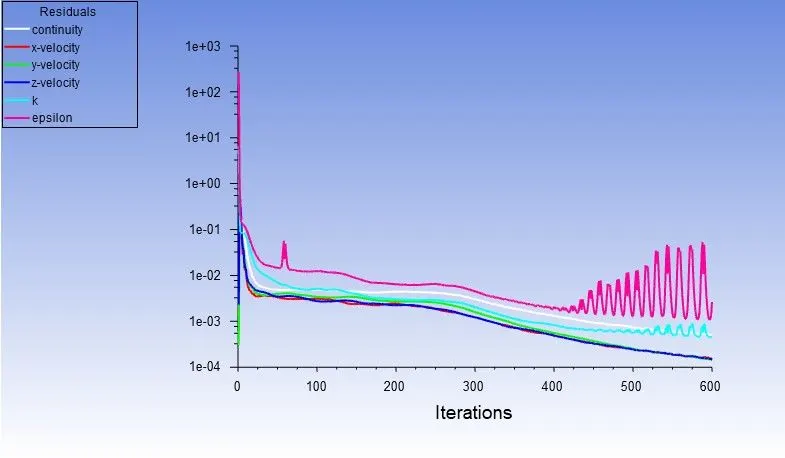
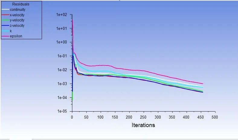
Now, under zones, we specify the boundary conditions for inlet and set velocity as 3m/s while specifying dpm as reflect for both inlet and walls. For outlet1 we set the dpm as escape and for outlet 2 as trap. Now, under solving, we choose standard method and using options we compute from the inlet and initialize the solution and run the solution for 450 iterations.

For 1`mu`m and v= 3m/s:

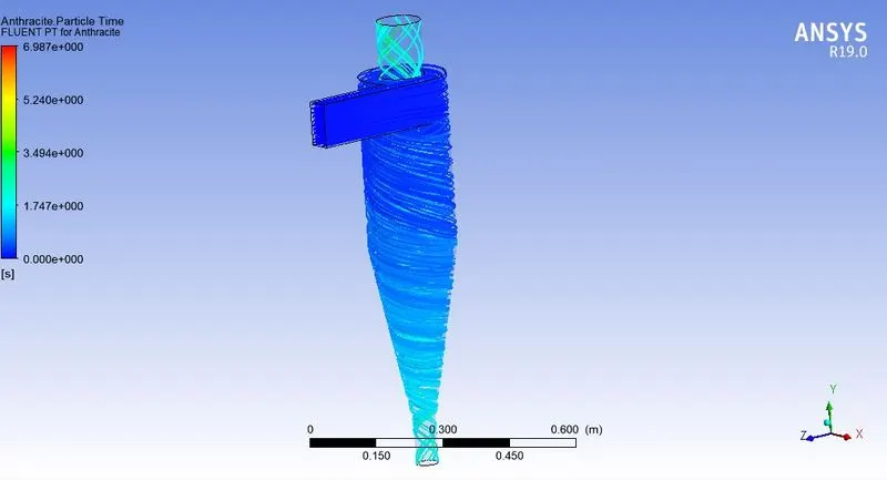
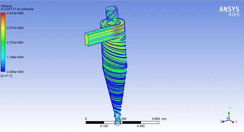
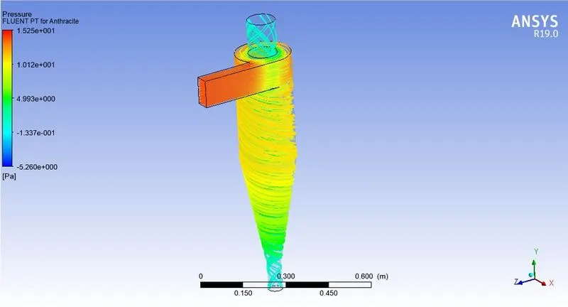
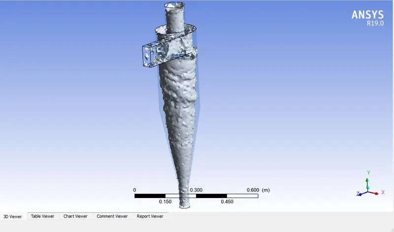
Separation efficiency: 32.25% (tracked 124; trapped 40)

For 5`mu`m and v = 3m/s:

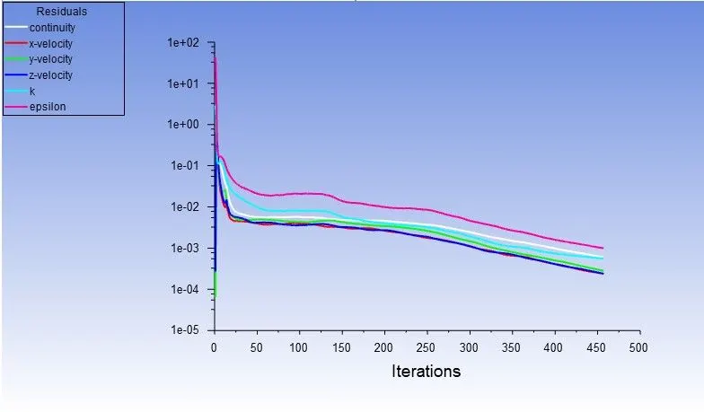
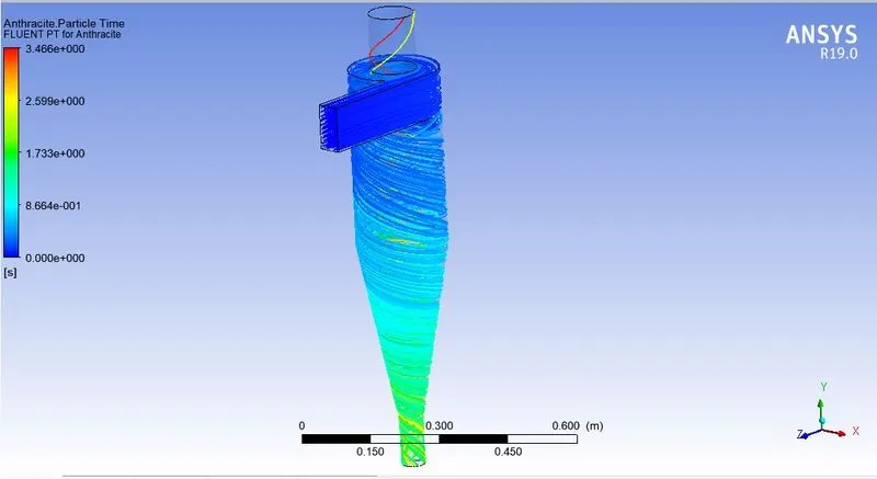
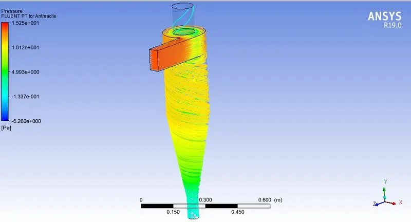
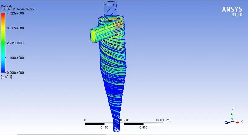
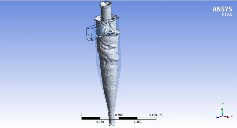
Separation efficiency: 64.51% (tracked 124; trapped 80)

For 5`mu`m and v=1m/s:

Separation efficiency: 27.41% (tracked 124; trapped 34)

For 5`mu`m and v = 5m/s:

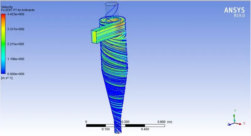
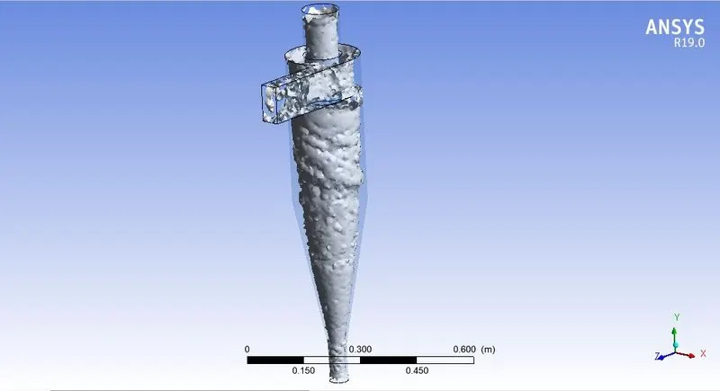
Separation efficiency: 56.45% (tracked 124; trapped 70)

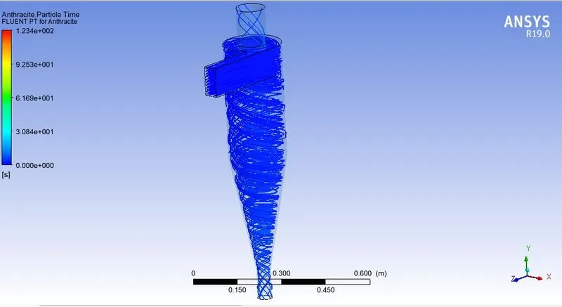
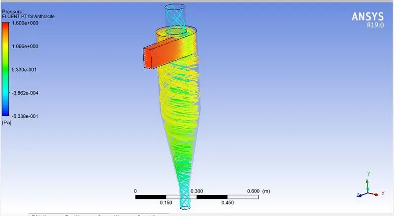
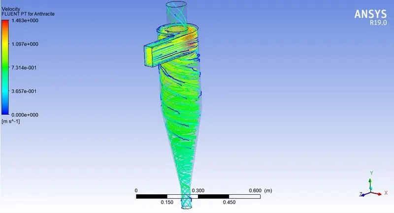
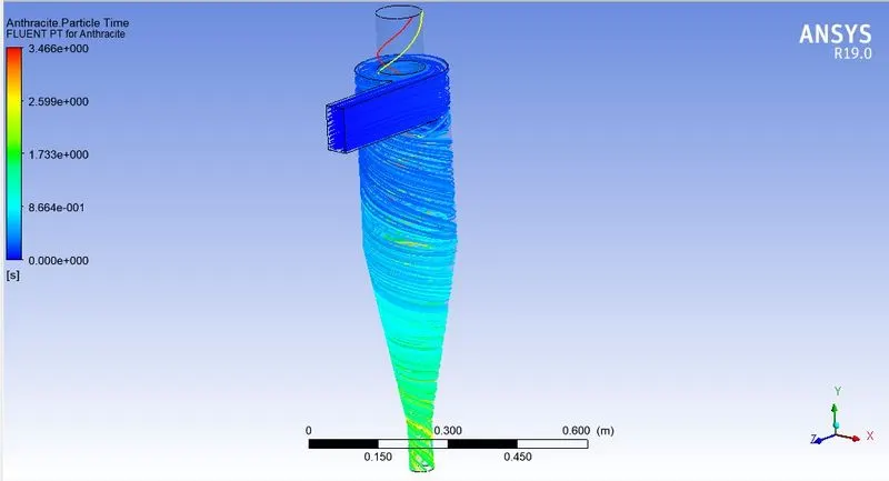
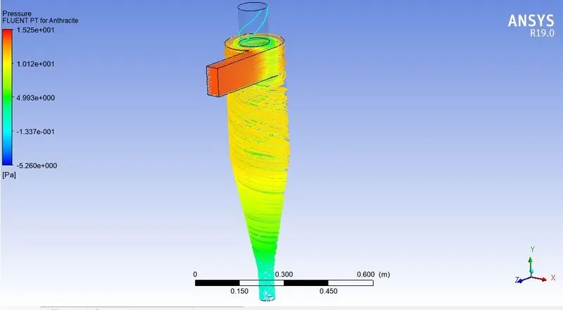
From the above plots, it is observed that for increase in size of the particles, the separator efficiency also increases and since the particles are blown out through the outlets, the negative sign in mass flow rate is observed. Also, for increase in both the particle as well as the inlet velocity, the separator efficiency increases.

It can be observed that not only from the main outlet, but some of the particles are shot out from the upper outlet as well.

The mass flow rates for all the cases are calculated as follows:

Mass flow rate	Inlet	Outlet
case 1	0.018375	-0.00293126
case 2	0.018375	-0.00293126
case 3	0.006125	-0.00116449
case 4	0.018375	-0.00293126