Week 3 - Solving second order ODEs

%second order differential equation

clear all
close all
clc

%factors needed
b = 0.05; %damping factor
g = 9.81; %gravitational constant
l = 1; %length of the string
m = 1; %mass of the object

% necessary initial conditions 
theta0 = [0;3];
time = linspace(0,20,100);

%function call
[t, rs] = ode45(@(t,theta) ode(t,theta,b,g,l,m), time, theta0);
    
    %plotting the reults
    plot(t, rs(:,1));
    hold on
    plot(t, rs(:,2));
    xlabel('Time');
    ylabel('Plot');
 
    %for animation of the pendulum
    ct = 1;
    for i = 1:length(time)
    x0 = 0;
    y0 = 0;
    x1 = l*sind(rs(i,1));
     y1 = l*cosd(rs(i,1));
     line([x0 x1],[y0,y1]);
      plot(x1,y1,'o','color','r');
     axis([-0.2 0.2 -0.3 1.2]);
     pause(0.005);
     M(ct) = getframe(gcf);
     ct = ct +1;
end

%creating a movie file
movie(M)
videofile = VideoWriter('Simple Pendulum','Uncompressed AVI');
open(videofile);
writeVideo(videofile,M);
close(videofile);







%function for solving second order ode
function [dthetadt] = ode(t,theta,b,g,l,m)

theta1 = theta(1);
theta2 = theta(2);
dtheta1dt = theta2;
dtheta2dt = -((b/m)*theta2)-(g/l)*sind(theta1);
dthetadt = [dtheta1dt; dtheta2dt];

end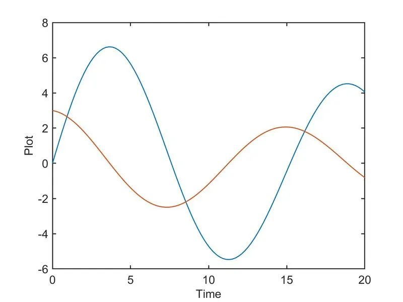

https://drive.google.com/file/d/1GsKf5Ogph1Ddtt98phB8BGwV-D0wEUU5/view?usp=drivesdk

For this challenge, we need to simulate the motion of a pendulum using animation in matlab. This is done by solving a second order ODE for a simple pendulum which is given as: d^2(theta)/dt^2 + b/m * dtheta/dt + g/l*sin(theta) = 0, where, b is the damping co-efficient, m is the mass of the bob, g is the gravitational acceleration and l is the length of the string.

We start by assuming the values for all the above mentioned factors. The initial condition here is that at time (t) = 0, the displacement is 0 and the angular velocity is 3 rad/sec. Similarly, the time span is given as 0-20 seconds and we use linspace command to get 100 values.

To solve the ODE, we need to know that the ODE is a function of theta and time. Therefore, we create a function named ODE where we get the result for dtheta/dt, which is a clubbed array of dtheta1/dt and dtheta1/dt. Since we have rewritten the formula for the simple pendulum in terms of theta1, theta2 as :

d/dt [theta1 theta2] = [theta2 -b/m*dtheta/dt-g/l*sin(theta)], where theta 1 = theta, theta2 = dtheta1/dt, we know that the function ODE is accepts values for time, theta, damping co-efficient, gravitational acceleration, length of string, mass of bob. Now we substitute the values for theta 1 and theta2 as theta(1) and theta(2) respectively, we can write theta as dtheta1/dt. similary, we can write the value for dtheta2/dt as -b/m * dtheta/dt - g/l*sin(theta) and finally, the result obtained from the function in the form of dtheta/dt is nothing but a matrix of 2 rows and one column with dtheta1/dt and dtheta2/dt as the values.

Now as we have to calculate the values for time and results, where results constitutes for the values of displacement and velocity, to solve the ODE, there is a matlab function ODE45 in which we can state what are the factors of which the ODE is a function of. In our case, our ODE is a function of time and theta, and we include the function ODE previously written along with the boundary conditions of time and intitial conditions at theta = 0.

Finally, we can plot the results for time vs diplacement and time vs velocity and save it. To create the animation for the pendulum, we need to include a for loop in the program. After assigning the value for the counter, We can provide a condition as for the value of i = length of the array time, the starting points of the string x0, y0 are at 0 position, i.e, disp =0. Now, we calculate the positions of the other end of the string by solving for sine and cosine of the angle made by the string with respect to the displacement made by the string at each iterations of time, i.e for each values of i ranging from 1-200. This is given as follows:

x1 = l*sind(rs(i,1));
y1 = l*cosd(rs(i,1));

Finally, we plot a line plot to visualize the string, plot the bob at the farthest end of the string using commands: line([x0 x1],[y0,y1]); plot(x1,y1,'o','color','r'). We set the axis scales, set a pause time of 0.05 seconds, create a variable M(ct) to capture the frames at each increment for ct.

Finally, we create a movie file named M using movie(M) command, videofile using videofile = VideoWriter('Simple Pendulum','Uncompressed AVI') with title of the file and the format, open the file, write the video into the file and close it using open(videofile),writeVideo(videofile,M), close(videofile) commands respectively.