Week 4.1 - Genetic Algorithm

%stalagmite function for global optimisation
clear all
close all
clc

%factors needed
x = linspace(0,2,200);
y = linspace(0,2,200);

%converting 1d array into 2d
[xx,yy] = meshgrid(x,y);

%evaluation of the stalagmite function 
for i = 1:length(xx)
    for j = 1:length(yy)
        ip(1) = xx(i,j);
        ip(2) = yy(i,j);
        f(i,j)= stalg(ip);
    end
end
%not bounded 
for i = 1:100
[inputs , fval(i)] = ga(@stalg,2);
xmax(i) = inputs(1);
ymax(i) = inputs(2);
end

figure(1);
subplot(2,1,1);
hold on
surf(x,y,f);
shading interp
plot3(xmax,ymax,-fval,'marker','o');
subplot(2,1,2);
hold on
plot(-fval);
xlabel('xvalue');
ylabel('yvalue');

%Bounded
for i = 1:100
[inputs , fval(i)] = ga(@stalg,2,[],[],[],[],[0;0],[2;2]);
xmax(i) = inputs(1);
ymax(i) = inputs(2);
end

figure(1);
subplot(2,1,1);
hold on
surf(x,y,f);
shading interp
plot3(xmax,ymax,-fval,'marker','o');
subplot(2,1,2);
hold on
plot(-fval);
xlabel('xvalue');
ylabel('yvalue');

%Bounded with increased initial population
optns=optimoptions('ga')
optns=optimoptions(optns,'populationsize',400);
for i = 1:100
[inputs , fval(i)] = ga(@stalg,2,[],[],[],[],[0;0],[2;2],[],[],optns);
xmax(i) = inputs(1);
ymax(i) = inputs(2);
end

figure(1);
subplot(2,1,1);
hold on
surf(x,y,f);
shading interp
plot3(xmax,ymax,-fval,'marker','o');
subplot(2,1,2);
hold on
plot(-fval);
xlabel('xvalue');
ylabel('yvalue');



%stalagmite
function [f] = stalg(ip)
x = ip(1);
y = ip(2);
f1x = (sind((5.1*pi*x)+0.5)).^6;
f1y = (sind((5.1*pi*y)+0.5)).^6;
f2x = exp(-4*log(2)*((x-0.0667).^2)/0.64);
f2y = exp(-4*log(2)*((y-0.0667).^2)/0.64);

f = -(f1x*f2x*f1y*f2y);

end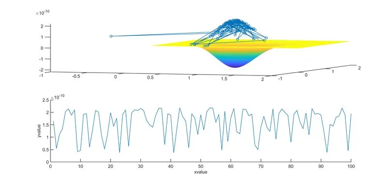

The aim here is to write a program for the stalagmite mathematical model for global optimisation problems. Optimisation is the process of minimising or maximising a function which is dependent upon multiple factors. So, a stalagmite function helps us to generate local minimas and maximas which helps us in the process of distinguishing.

We start with 2 variables and assign each of them multiple values in the form of an array following by converting them into 3 dimensional arrays using meshgrid. Now, we evaluate the stalagmite function using a for loop by first assigning initial conditions for loop, for the variables xx and yy, storing the values of xx and yy in new arrays for each iterations of i and j, and calling the function, called stalg to get the input variables. The stalg function is dependent upon 2 variables x and y, and to generate the stalagmite functions, the equztions used are as follows:

f1x=[sin(5.1*pi*x+0.5)]^6
f1y=[sin(5.1*pi*y+0.5)]^6
f2x=exp(−4log(2)*(x−0.0667)^2)/0.64
f2y=exp(−4log(2)*(y−0.0667)^2)/0.64

f(x,y) = f1x+f2x+f1y+f2y

Now the first condition is to analyse the output of the stalagmite function for no boundary conditions. We set the number of iterations of the loop, store the values for inputs and fval in an array which is the genetic algorithm function operated with the stalagmite function and the number of variables the function is dependent upon. The genetic algorithm (ga) is an inbuilt matlab function used to choose only the fittest values for performing the operation. Random values are chosen and the default results obtained are minimum values. So, in order to get the maximum values, we assign negative value for the stalagmite function output. We plot the values using surface plot, use shading interp command to smoothen and get rid of lines in the plot, plot the xmax, and y max values along with fval.

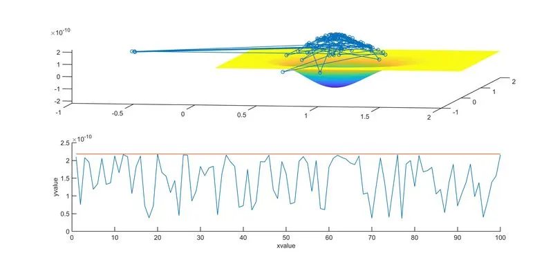
Again =, we try to run the code but now, we provide boundary conditions in the form of limits for x and y values. So, we use ga(@stalg,2,[],[],[],[],[0;0],[2;2]); where [] indicates whether the function is subjected to linear inequalities, evaluates and assigns the values accordingly, the lower bound and upper bound values. Now, the resullts we obtain are constrained values, but still scattered multiple values.

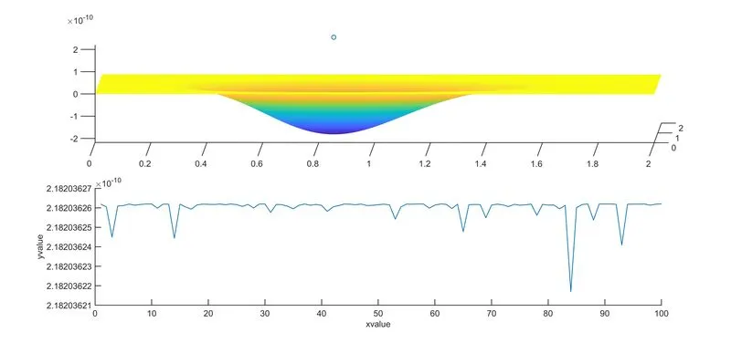
Finally, we try using boundary condition along with the given condition of initial population number. This is done using: optns=optimoptions('ga')
optns=optimoptions(optns,'population',400); which sets the value for the initial population from the given condition. We can increase the iterations to narrow up the values and get accurate results. The algorithm for this program terminates when the values have converged. Now, the results show the exact value for the maxima.