Week 3.5 - Deriving 4th order approximation of a 2nd order derivative using Taylor Table method

Here, for fourth order approximation of a second order derivative, we use two methods, central differencing scheme and skewed scheme. It is given that p = n-q+1 for central difference scheme and p = n-q for one sided schemes, where p is the order of the derivative, q is the order of approximation and n is the number of nodes.

First, for the central difference scheme, number of nodes (n) = p+q-1 => 2+4-1 = 5.

`(del^2f)/(delx^2) = (a.f(i-2)+b.f(i-1)+c.fi+d.f(i+1)+e.f(i+2))/dx^2` and using taylor series expansion method, for the first node: `a.f(i-2) = a.f(i) - 2a. (f'(i)dx)/(1!) + 4a.(f''(i)dx^2)/(2!)-8a.(f'''(i)dx^3)/(3!)+16a.(f''''(i)dx^4)/(4!)`.

Similarly, using taylor series expansion method, after expanding all the terms and reassembling them in a table, we get:

	`f(i)`	`f'(i)dx`	`f''(i).dx^2`	`f'''(i).dx^3`	`f''''(i)dx^4`
`a.f(i-2)`	`a`	`-2a`	`2a`	`-(4a)/3`	`(2a)/3`
`b.f(i-1)`	`b`	`-b`	`b/2`	`-b/6`	`b/24`
`c.f(i)`	`c`	`0`	`0`	`0`	`0`
`d.f(i+1)`	`d`	`d`	`d/2`	`d/6`	`d/24`
`e.f(i+2)`	`e`	`2e`	`2e`	`(4e)/3`	`(2e)/3`
`sum`	`0`	`0`	`1`	`0`	`0`

Now, we can form matrices from the above values as:

`[[1,1,1,1,1],[-2,-1,0,1,2],[2,1/2,0,1/2,2],[-4/3,-1/6,0,1/6,4/3],[2/3,1/24,0,1/24,2/3]].[[a],[b],[c],[d],[e]]=[[0],[0],[1],[0],[0]]`

This matrix can be used to find the inverse of matrix A which is the 4x5 matrix and solved to get the coefficient matrix. The coefficients a,b,c,d,e obtained respectively are:

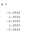
We substitute these values in the equation we ealier derived. Similarly, for right skew,

`(del^2f)/(delx^2) = (a.f(i)+b.f(i+1)+c.f(i+2)+d.f(i+3)+e.f(i+4)+m.f(i+5))/(dx^2)` for number of nodes (n) = p+q = 2+4 = 6 and for left skew`

`(del^2f)/(delx^2) = (a.f(i-5)+b.f(i-4)+c.f(i-3)+d.f(i-2)+e.f(i-1)+m.f(i))/(dx^2)`

Performing similar actions like in central difference scheme, we obtain all the coefficients and substitute them in the respective derived equations. Now, the analytical function given is : `exp(x)*cos(x)`. The analytical derivative will be : `-2.exp(x).sin(x)`

%4th order approximation for a second order derivative
clear all
close all
clc

%parameters needed
x = pi/3;
dx = linspace(pi/4000,pi/40,100);

%calling functions
for i = 1:length(dx)
cde(i) = cds(x,dx(i));
rse(i) = rss(x,dx(i));
lse(i) = lss(x,dx(i));
end

%plotting
figure(1);
loglog(dx,cde,'r');
hold on
loglog(dx,rse,'g');
hold on
loglog(dx,lse,'b');
xlabel('order of approximation');
ylabel('error');
legend('Central difference','RIght skew','Left skew');


%function central difference scheme
function out = cds(x,dx)

ad = -2*exp(x)*sin(x);
cd = (((-0.0833)*((exp(x-(2*dx)))*(cos(x-(2*dx)))))+((1.3333)*((exp(x-dx))*(cos(x-dx))))-((2.5000)*((exp(x))*(cos(x))))+((1.3333)*((exp(x+dx))*(cos(x+dx))))-((0.0833)*((exp(x+(2*dx)))*(cos(x+(2*dx))))))/(dx^2);

out = abs(cd - ad);
end


%function right skew scheme
function out = rss(x,dx)

ad = -2*exp(x)*sin(x);
rd = (((3.7500)*((exp(x))*(cos(x))))-((12.8333)*((exp(x+dx))*(cos(x+dx))))+((17.8333)*((exp(x+(2*dx)))*(cos(x+(2*dx)))))-((13.0000)*((exp(x+(3*dx)))*(cos(x+(3*dx)))))+((5.0833)*((exp(x+(4*dx)))*(cos(x+(4*dx)))))-((0.8333)*((exp(x+(5*dx)))*(cos(x+(5*dx))))))/(dx^2);
out = abs(rd - ad);
end


%function left skew scheme
function out = lss(x,dx)

ad = -2*exp(x)*sin(x);
ld = (((-0.8333)*((exp(x-(5*dx)))*(cos(x-(5*dx)))))+((5.0833)*((exp(x-(4*dx)))*(cos(x-(4*dx)))))-((13.0000)*((exp(x-(3*dx)))*(cos(x-(3*dx)))))+((17.8333)*((exp(x-(2*dx)))*(cos(x-(2*dx)))))-((12.8333)*((exp(x-dx))*(cos(x-dx))))+((3.7500)*((exp(x))*(cos(x)))))/(dx^2);
out = abs(ld - ad);
end

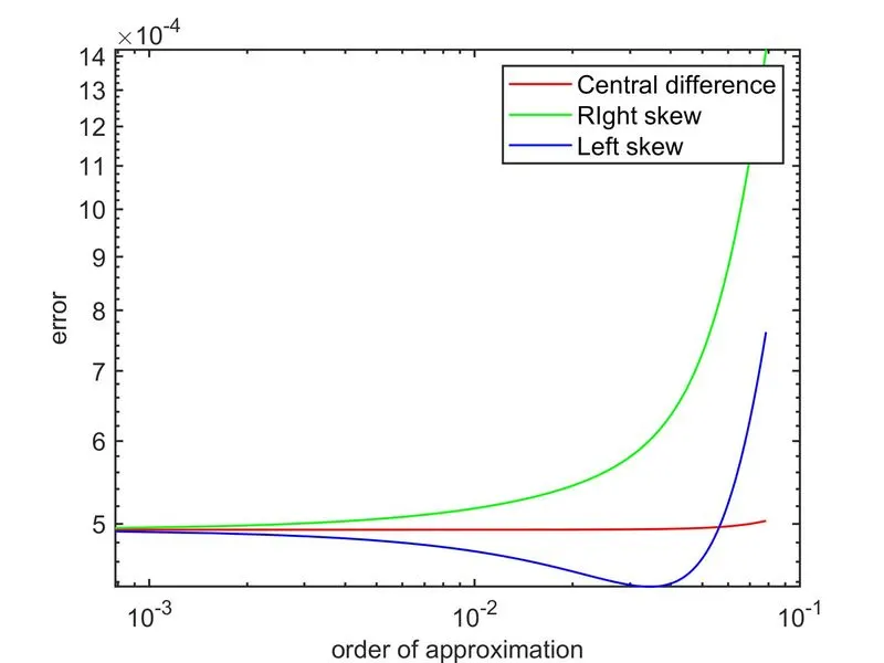
From the plot obtained, it is evident that the error for central difference scheme is less and it is why it is prefferred for second order derivatives. But, there are conditions where there are less data available at both the ends, and therefore, central difference method cannot be utilised. Also, at the boundary nodes, where the immediate availability for left and right points are not possible, central difference scheme cannot be useful. Therefore, skewed scheme can be used.