Week 8 - Simulating Cyclone separator with Discrete Phase Modelling
AIM:- The project aim is to perform an analysis of the cyclone separator and calculate the separation efficiency and pressure drop.
OBJECTIVE:- The project objectives are-
- To write a few words about any four empirical models used to calculate the cyclone separator efficiency.
- To perform an analysis on a given cyclone separator model by varying the particle diameter from 1 μm to 5 μm and calculating the separation efficiency in each case. Discuss the results. [Use both the velocity's as 3m/sec.]
- To perform an analysis on a given cyclone separator model by varying the particle velocity from 1 m/sec to 5 m/sec and calculate the separation efficiency and pressure drop in each case. Discuss the results. [Use particle diameter size as 5 μm for all cases & keep flow velocity the same as particle velocity]
INTRODUCTION:- Cyclones are devices that employ a centrifugal force generated by spinning gas steam to separate particles from the carrier gas. A gas cyclone separator is widely used in industries to separate dust from gas or for product recovery because of its geometrical simplicity, the relative economy in power, and flexibility.
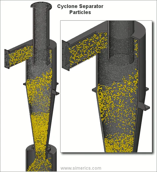
This figure shows how we separate smaller particle from bigger particle.
Cyclones are particularly well suited for high temperature and pressure conditions because of their rugged design and flexible component materials and they can be operated at very high dust loading. Cyclone separators are used for the removal of large particles for both air pollution control and process use. Application in extreme conditions includes the removal of coal dust in a power plant and the use as a spray dryer or gasification reactor.
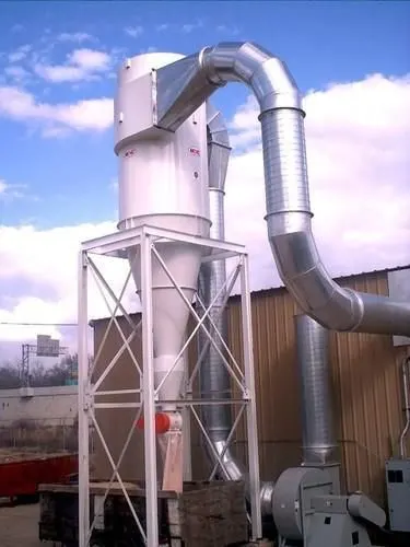
Fig: Industrial Cyclone Separator
Engineers are generally interested in two parameters to assess the design and performance of a cyclone. These parameters are the cyclone efficiency of particles and pressure drop through the cyclone. An accurate prediction of cyclone efficiency is very important because inaccuracy in the efficiency prediction may result in an inefficient design of the cyclone separator. CFD has a great potential to predict the flow field characteristics and particle trajectories inside the cyclone. The complicated swirling turbulent flow in a cyclone places great demands on the numerical techniques and the turbulence models employed in the CFD codes when modeling the cyclone pressure drop.
This study presents an application of CFD, in the prediction of cyclone efficiency. This study also reviews the four empirical models for cyclone efficiency. Additionally, we can analyze simulation results. Our simulation can be done in Ansys Fluent.
PROJECT DESCRIPTION:- Before going to our simulation, let's discuss four empirical models to calculate cyclone separator efficiency-
- Iozia and Leith Model:-Iozia and Leith logistic model is a modified version of the Barth Model, which is developed based on force balance. The model assumes that a particle carried by the vortex endures the influence of two forces: a centrifugal force, Z, and flow resistance, W. The collection efficiency `eta_i` of particle diameter `d_"pi"`can be calculated from
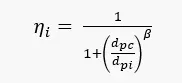
`beta` is an expression for slope parameter derived based on the statistical analysis of experimental data of a cyclone with D = 0.25 m gives as

And dpc is the 50% cut size given by Bath
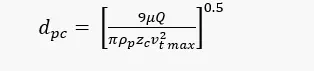
Where core length, zc, and core diameter, dc, are given as

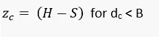
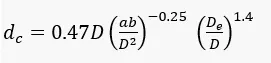
-
Li and Wang Model:- The Li and Wang model includes particle bounce or re-entrainment and turbulent diffusion at the cyclone wall. A two-dimensional analytical expression of practical distribution in the cyclone is obtained. Li and Wang's model was developed based on the following assumptions:
- The radial particle velocity and the radial concentration profile are not constant for uncontrolled particles within the cyclone.
- Boundary conditions with the consideration of turbulent diffusion coefficient and particle bounce reentrainment on the cyclone wall are:
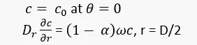
- The tangential velocity is related to the radius of the cyclone by uRn = constant.
The concentration distribution in a cyclone is given as:
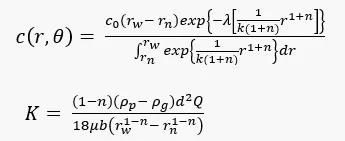
And
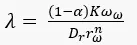
The resultant expression of the collection efficiency for a particle of any size is given as

Where

-
Koch and Licht Model:- Koch and Licht's collection theory recognized the inherently turbulent nature of cyclones and the distribution of gas residence times within the cyclone. Koch and Licht described particle motion in the entry and collection regions with the additional following assumptions:
- The tangential velocity of a particle is equal to the tangential velocity of the gas flow, there is no slip in the tangential direction between the particle and the gas.
- The tangential velocity is related to the radius of the cyclone by uRn = constant.
A force balance and an equation on the particles collection yield the grade efficiency `eta_i`
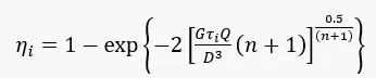
Where
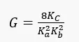

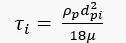
G is a factor related to the configuration of the cyclone, n is the related to the vortex and `tau` is the relaxation term.
-
Lapple Model:- Lapple model was developed based on the force balance with our considering the flow resistance. Lapple assumed that a particle entering the cyclone is evenly distributed across the inlet opening. The particle that travels from the inlet half width to the wall in the cyclone is collected with 50% efficiency. The semi-empirical relationship developed by Lapple to calculate a 50% cut diameter, dpc, is
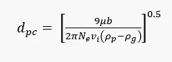
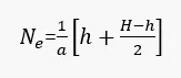
Where is the number of revolutions
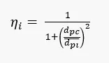
The efficiency of collection of any size of a particle is given by
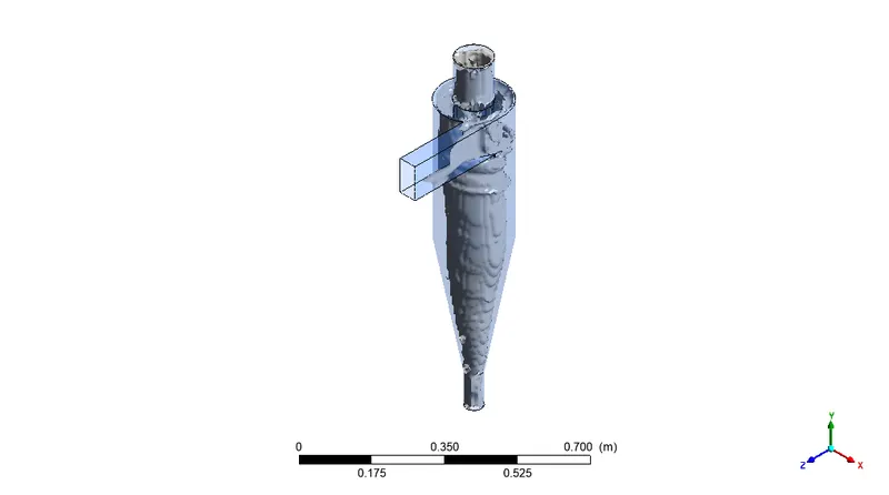
Geometry and Meshing:- This is our geometry -
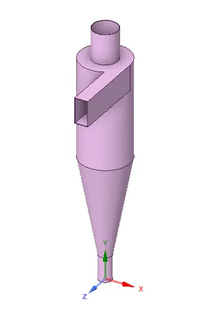
To extract the fluid volume from the geometry we use the Volume Extract tool in the Analysis group on the Prepare tab and select the edges to enclose the region.
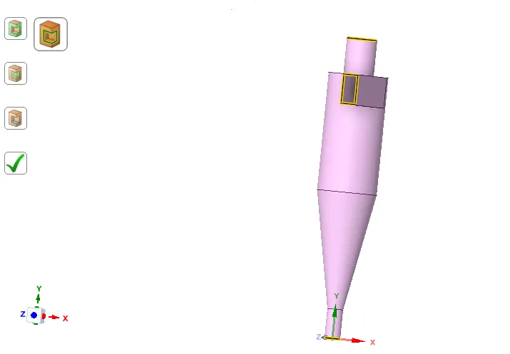
Now we created the fluid volume
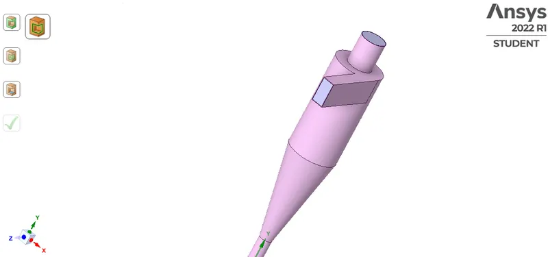
After creating fluid volume, we hide our geometry. Since it can effect the analysis, we select the geometry and click on suppress for physics option.
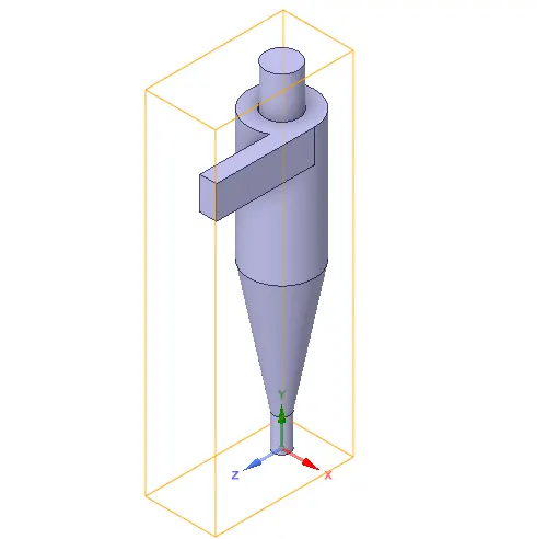
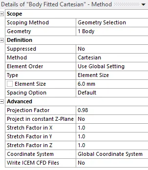
Meshing:- Here we use Body fitted cartesian meshing for more accurate result.
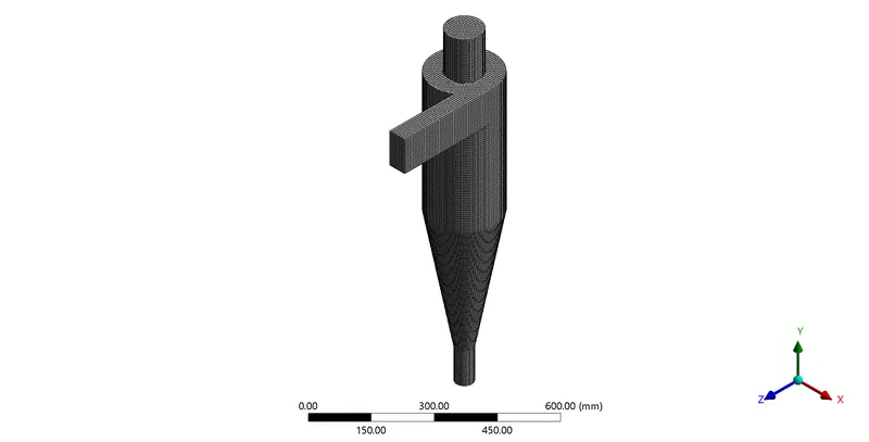
Mesh details:-

Solver Settings:-
- Pressure-based solvers and absolute velocity are used.
- It is a 3D simulation.
- Steady-state simulation is performed.
- The gravity is enabled in the -ve Y-axis.
- The RNG K-epsilon turbulence model is taken as a viscous model. Because the RNG model is better for swirling flow.
- Here we use Discrete phase modeling. Discrete phase models are used in simulating dilute particle flows. In these methods, point masses that are representing parcels of particles are traced through the computational domain by evaluating local force balances.
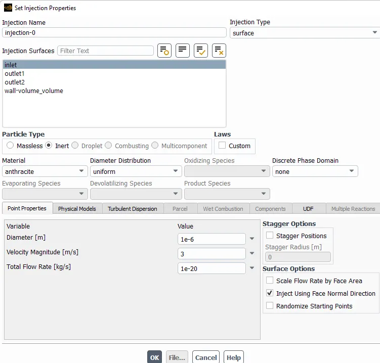
- Here we take inert particle as Anthracite. We inject Anthracite through inlet face and we keep both the velocity same.
- In pressure-velocity coupling, a SIMPLE scheme is used. For the momentum, a second order upwind scheme is used and for pressure, the second order is selected. In the case of Turbulent Kinetic Energy and Turbulent Dissipation Rate, a second-order scheme is chosen.
Report:- This is one of the simulation full report
Fluent
Version: 3d, dp, pbns, rngke (3d, double precision, pressure-based, RNG k-epsilon)
Release: 22.1.0
Title:

Models
------

   Model                              Settings
   -----------------------------------------------------------------
   Space                              3D
   Time                               Steady
   Viscous                            RNG k-epsilon turbulence model
   Wall Treatment                     Standard Wall Functions
   RNG Differential Viscosity Model   Disabled
   RNG Swirl Dominated Flow Option    Enabled
   Heat Transfer                      Disabled
   Solidification and Melting         Disabled
   Species                            Disabled
   Coupled Dispersed Phase            Enabled
   NOx Pollutants                     Disabled
   SOx Pollutants                     Disabled
   Soot                               Disabled
   Mercury Pollutants                 Disabled
   Structure                          Disabled
   Acoustics                          Disabled
   Eulerian Wall Film                 Disabled
   Potential/Li-ion Battery           Disabled
   Multiphase                         Disabled


Material Properties
-------------------

   Material: anthracite (inert-particle)

      Property             Units      Method     Value(s)
      ---------------------------------------------------
      Density              kg/m^3     constant   1550
      Cp (Specific Heat)   J/(kg K)   constant   1680

   Material: air (fluid)

      Property                        Units      Method     Value(s)
      ----------------------------------------------------------------
      Density                         kg/m^3     constant   1.225
      Cp (Specific Heat)              J/(kg K)   constant   1006.43
      Thermal Conductivity            W/(m K)    constant   0.0242
      Viscosity                       kg/(m s)   constant   1.7894e-05
      Molecular Weight                kg/kmol    constant   28.966
      Thermal Expansion Coefficient   K^-1       constant   0
      Speed of Sound                  m/s        none       #f

   Material: aluminum (solid)

      Property               Units      Method     Value(s)
      -----------------------------------------------------
      Density                kg/m^3     constant   2719
      Cp (Specific Heat)     J/(kg K)   constant   871
      Thermal Conductivity   W/(m K)    constant   202.4


Cell Zone Conditions
--------------------

   Zones

      name            id   type
      --------------------------
      volume_volume   3    fluid

   Setup Conditions

      volume_volume

         Condition       Value
         ---------------------
         Frame Motion?   no


Boundary Conditions
-------------------

   Zones

      name                 id   type
      -----------------------------------------
      wall-volume_volume   1    wall
      inlet                6    velocity-inlet
      outlet1              7    pressure-outlet
      outlet2              8    pressure-outlet

   Setup Conditions

      wall-volume_volume

         Condition                  Value
         ------------------------------------------
         Wall Motion                Stationary Wall
         Shear Boundary Condition   No Slip

      inlet

         Condition                  Value
         ----------------------------------
         Velocity Magnitude [m/s]   3
         Discrete Phase BC Type     reflect

      outlet1

         Condition   Value
         -----------------

      outlet2

         Condition                Value
         ------------------------------
         Discrete Phase BC Type   trap


Solver Settings
---------------

   Equations

      Equation     Solved
      -------------------
      Flow         yes
      Turbulence   yes

   Numerics

      Numeric                         Enabled
      ---------------------------------------
      Absolute Velocity Formulation   yes

   Under-Relaxation Factors

      Variable                     Relaxation Factor
      ----------------------------------------------
      Pressure                     0.3
      Density                      1
      Body Forces                  1
      Momentum                     0.7
      Turbulent Kinetic Energy     0.8
      Turbulent Dissipation Rate   0.8
      Turbulent Viscosity          1
      Discrete Phase Sources       0.5

   Linear Solver

      Variable                     Solver Type   Termination Criterion   Residual Reduction Tolerance
      -----------------------------------------------------------------------------------------------
      Pressure                     V-Cycle       0.1
      X-Momentum                   Flexible      0.1                     0.7
      Y-Momentum                   Flexible      0.1                     0.7
      Z-Momentum                   Flexible      0.1                     0.7
      Turbulent Kinetic Energy     Flexible      0.1                     0.7
      Turbulent Dissipation Rate   Flexible      0.1                     0.7

   Pressure-Velocity Coupling

      Parameter   Value
      ------------------
      Type        SIMPLE

   Discretization Scheme

      Variable                     Scheme
      ------------------------------------------------
      Pressure                     Second Order
      Momentum                     Second Order Upwind
      Turbulent Kinetic Energy     Second Order Upwind
      Turbulent Dissipation Rate   Second Order Upwind

   Solution Limits

      Quantity                         Limit
      ---------------------------------------
      Minimum Absolute Pressure        1
      Maximum Absolute Pressure        5e+10
      Minimum Temperature              1
      Maximum Temperature              5000
      Minimum Turb. Kinetic Energy     1e-14
      Minimum Turb. Dissipation Rate   1e-20
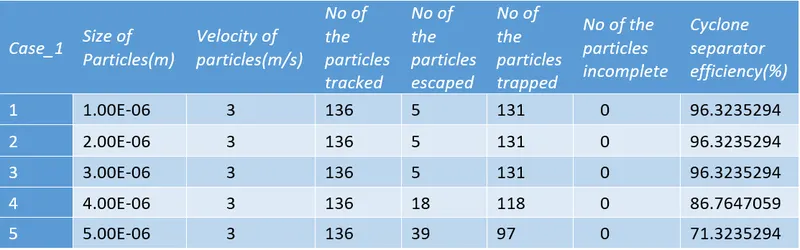
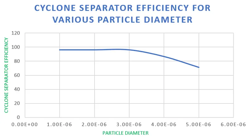
Maximum Turb. Viscosity Ratio 100000 CASE_1:- In case 1, we perform an analysis on a given cyclone separator model by varying the particle diameter from 1 μm to 5 μm and calculate the separation efficiency in each case. And we also discuss the results. Here we use both the velocity's as 3m/sec for all five simulations.
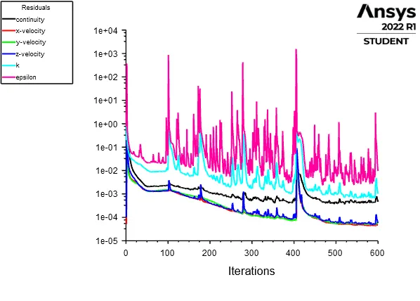
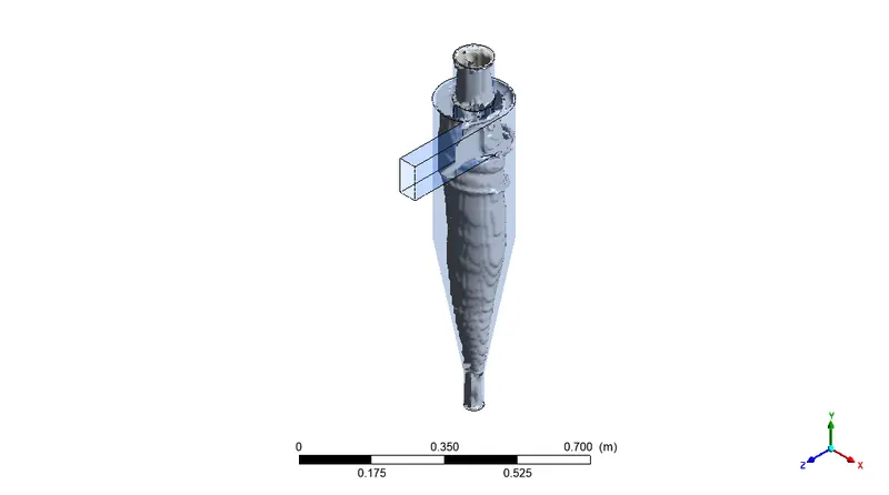
Results for 1μm:-
Residual:-
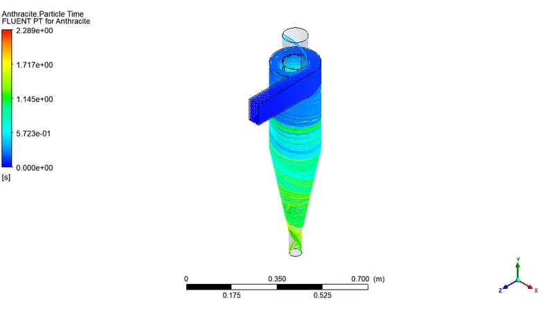
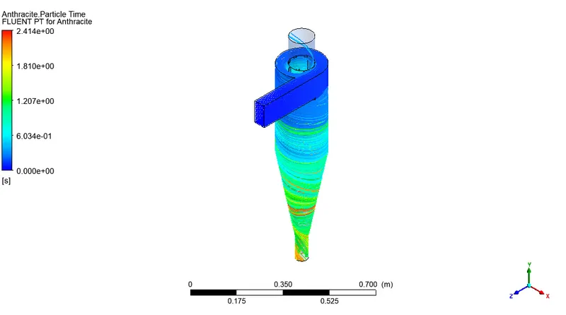
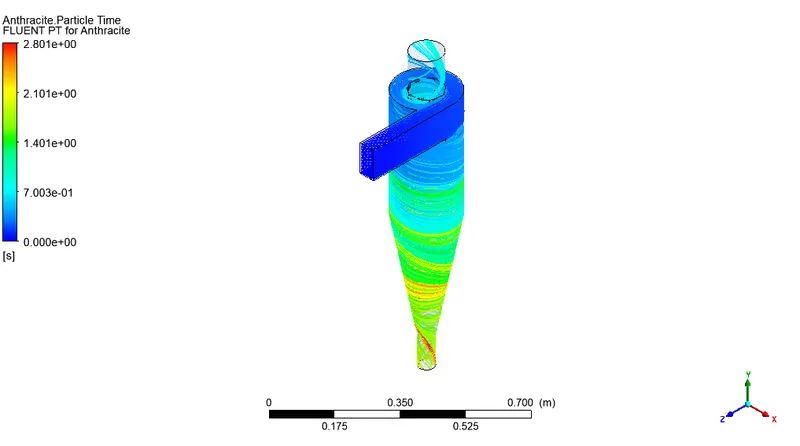
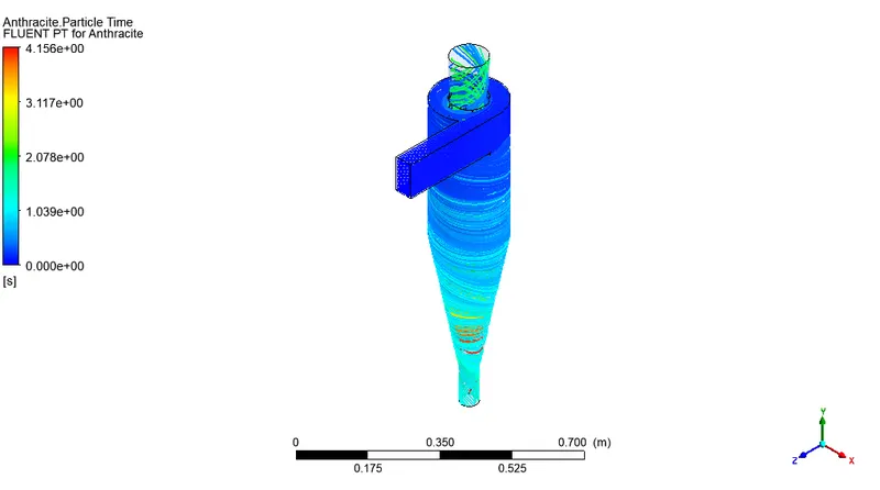
Anthracite Particle Time Plot:-
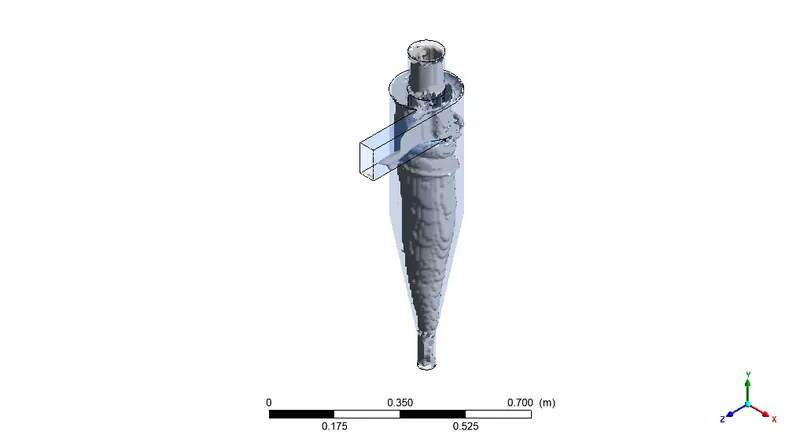
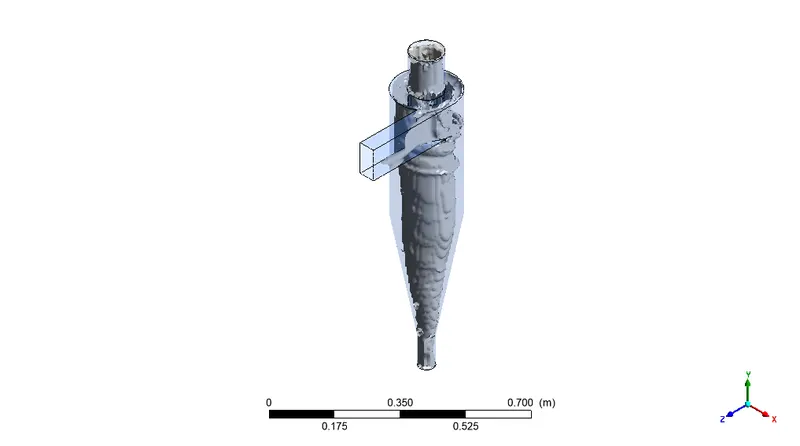
Vortex Core Region:-
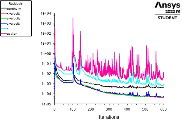
Results for 2μm:-
Residual:-
Anthracite Particle Time Plot:-
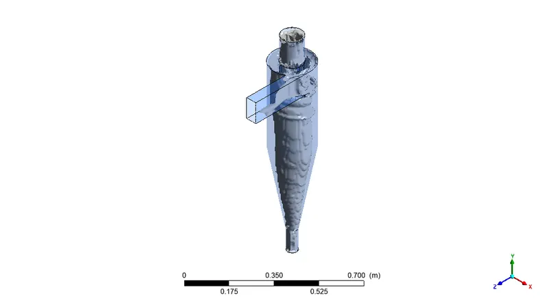
Vortex Core Region:-
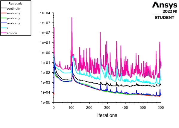
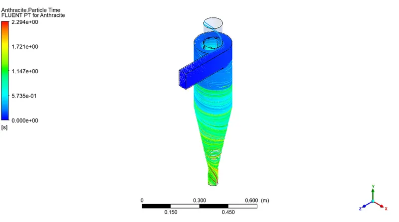
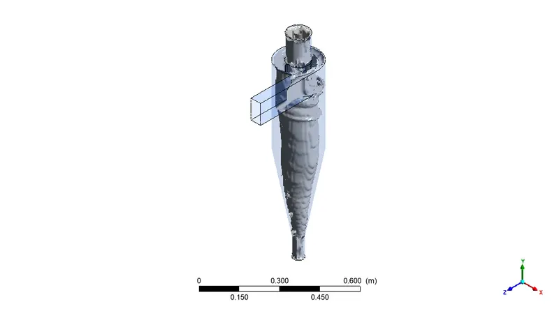
Results for 3μm:-
Residual:-
Anthracite Particle Time Plot:-
Vortex Core Region:-
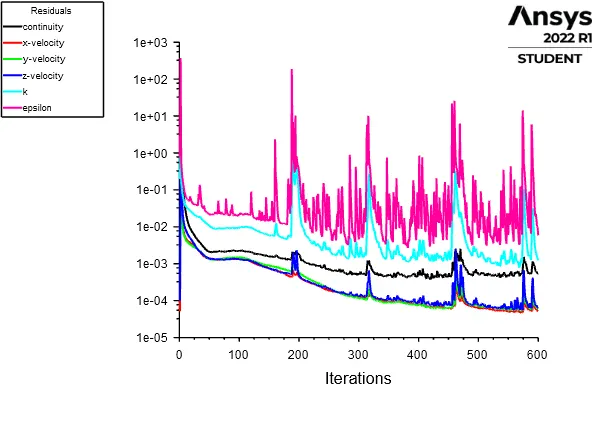
Results for 4μm:-
Residual:-
Anthracite Particle Time Plot:-
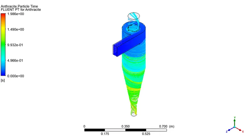
Vortex Core Region:-
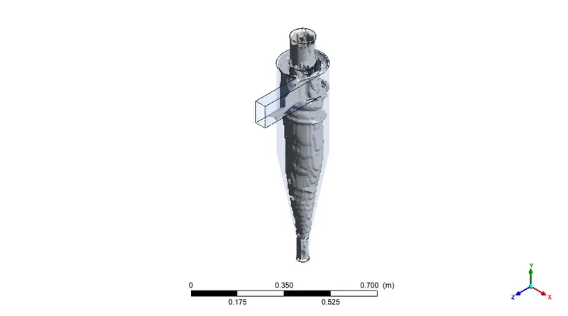
Results for 5μm:-
Residual:-
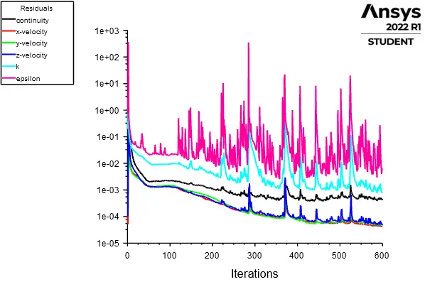
Anthracite Particle Time Plot:-
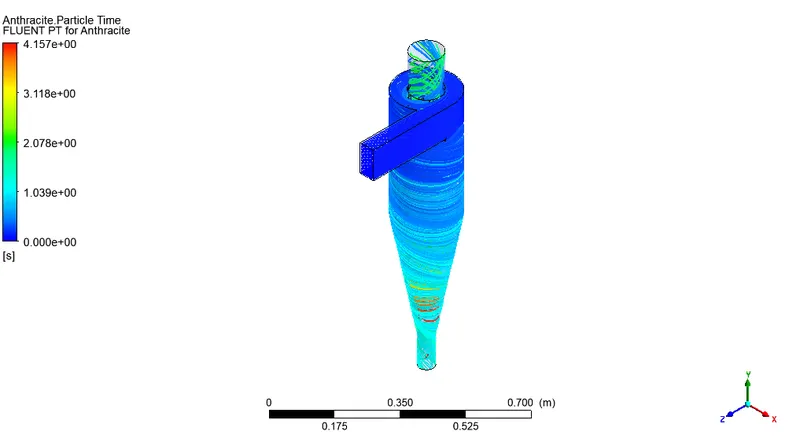
Vortex Core Region:-
Data Table for the results for various particle diameter:-
Cyclone Separator efficiency vs Particle Diameter Plot:-
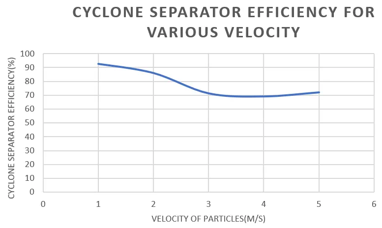
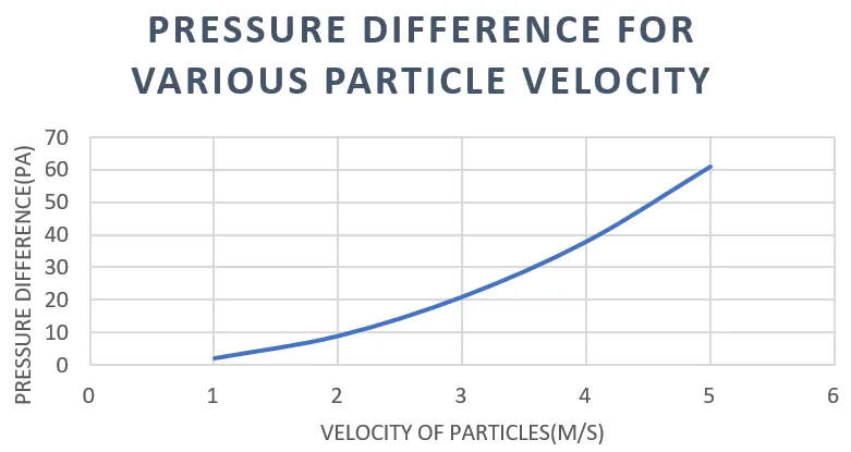
CASE_2:- In case 2, we perform an analysis on a given cyclone separator model by varying the particle velocity from 1 m/sec to 5 m/sec and calculate the separation efficiency and pressure drop in each case.. And we also discuss the results. Here we use particle diameter size as 5 μm for all five simulations.
Results for 1m/s:-
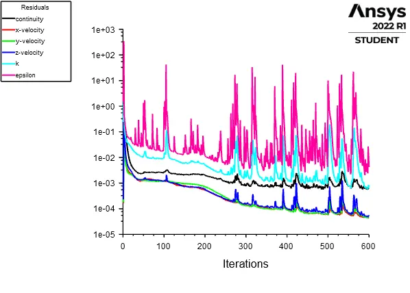
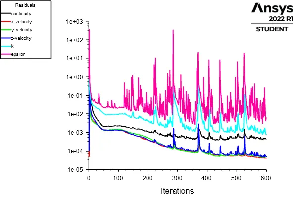
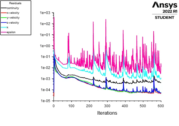
Residual:-
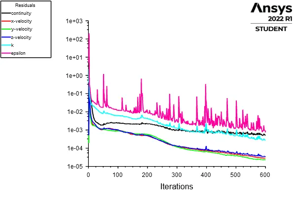
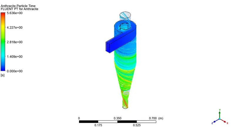
Anthracite Particle Time Plot:-
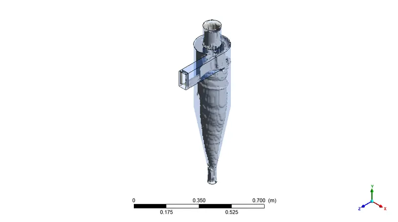
Vortex Core Region:-
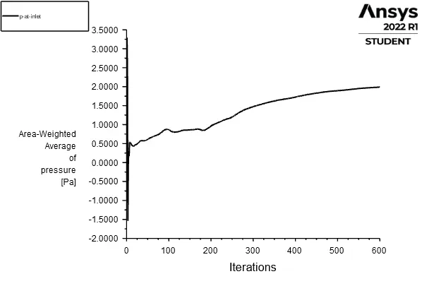
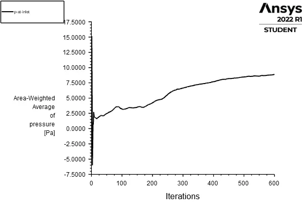
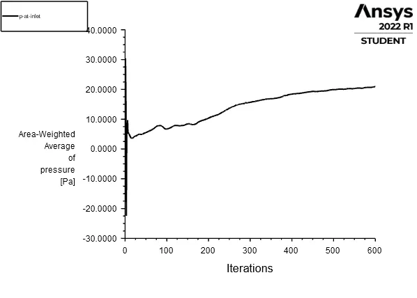
Inlet Pressure:-
Results for 2m/s:-
Residual:-
Anthracite Particle Time Plot:-
Vortex Core Region:-
Inlet Pressure:-
Results for 3m/s:-
Residual:-
Anthracite Particle Time Plot:-
Vortex Core Region:-
Inlet Pressure:-
Results for 4m/s:-
Residual:-
Anthracite Particle Time Plot:-
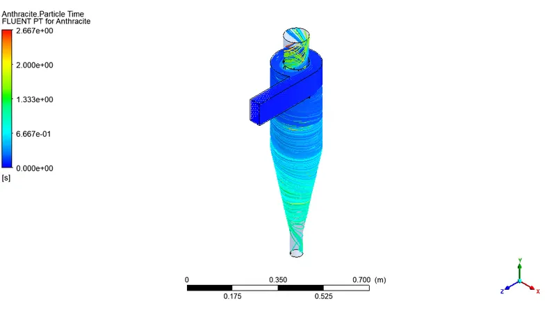
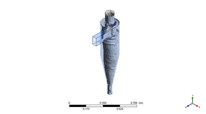
Vortex Core Region:-
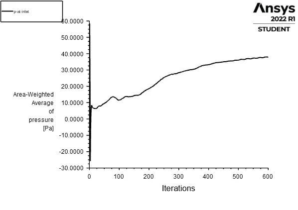
Inlet Pressure:-
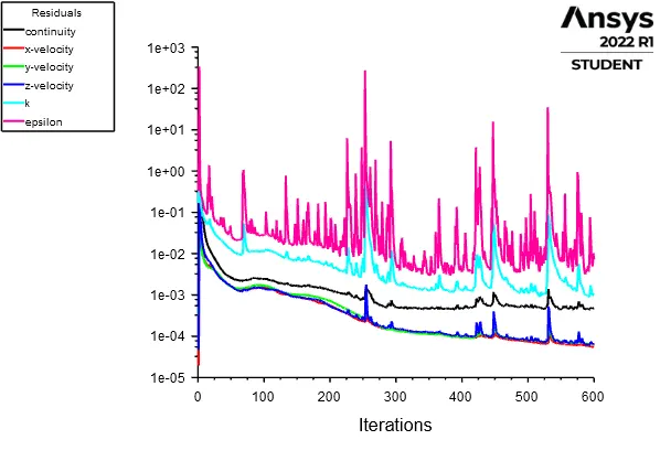
Results for 5m/s:-
Residual:-
Anthracite Particle Time Plot:-
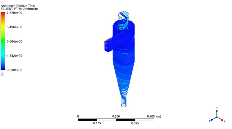
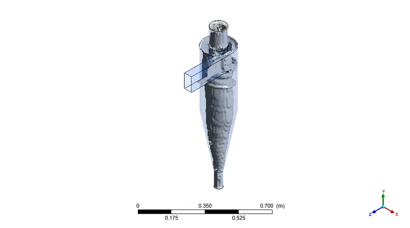
Vortex Core Region:-
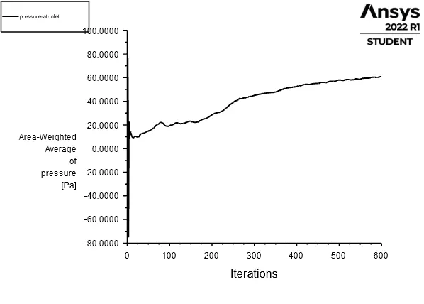
Inlet Pressure:-
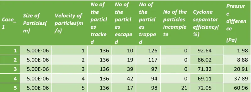
Data Table for the results for various velocity:-
Cyclone Separator efficiency vs Particle Velocity Plot:-
Pressure Difference vs Particle Velocity Plot:-
CONCLUSION:- After seeing all the result we conclude that -
- With the increase of particle diameter, the efficiency will decrease.
- With the increase of particle velocity, the efficiency will decrease.
- With the increase of particle velocity, the Pressure will increase.