Dynamic Mesh Simulation of Gear-Box with Volume of Fluid Method

Aim:

In this challenge, we are going to simulate a gearbox. To simulate the gearbox we will be using a dynamic meshing approach in Ansys Fluent.

Introduction:

Dynamics meshing means when the mesh is updated every time step. Dynamic meshing is used when there is boundary motion, such as valves, store separation, ships in the sea. There are three methods available in Ansys Fluent to perform dynamic meshing simulation. They are - Layering, Smoothing, Remeshing.

1. Layering:
Layering is most useful for linear motion and pure rotational motion.
Layering involves the creation and destruction of cells
– Cells are added as the zone grows.
– Cells are deleted as the zone shrinks.
– Cells connectivity change.

Requires the cell shapes of
Quad elements: 2D
Wedge, Hexa elements: 3D

2. Smoothing:
The smoothing method moves interior nodes to absorb the motion of a moving/deforming boundary. The number of nodes and their connectivity does not change.
Two different smoothing methods are available
for interior zones:

Spring-based smoothing: Spring/Laplace/Boundary Layer
The edges between any two nodes are idealized as a network of springs. A displacement at a boundary node will generate a “spring force”.

Diffusion – based smoothing:
The mesh motion is governed by the diffusion equation.
Diffusion-based smoothing is generally more computationally costly than spring-based smoothing but tends to generate better quality meshes. Allows larger deformations than spring-based smoothing.

3. Remeshing:
The remeshing method makes it possible to simulate problems with the large relative motion of boundaries.
‒ Cells and faces are remeshed when skewness or size
exceeds specified limits.
‒ The number of nodes and their connectivity changes
as cells/faces are added or deleted.

Available remeshing methods:
i) Local cell = Remesh interior cells (2D & 3D)
ii) Zone remeshing = Remesh the complete cell zone if local remeshing fails (2D & 3D)
iii) Local face = Remesh tri faces on deforming boundaries (only for 3D)
iv) Region face = Remesh faces adjacent to a moving boundary (2D & 3D)
v) 2.5D = Remesh prisms elements in 3D zones (prisms from extruded tri elements)
vi) Cutcell zone = Remesh cells & faces of a complete zone

Fluid Sloshing:

Sloshing is caused by the forces acting on the liquid, which change their magnitude and orientation relative to the tank during the time.

Effects of Sloshing-
- Energy loss due to the motion of the liquid fuel affects the gyroscopic stability of the spacecraft and leads to the nutation (wobble).
- Strong impact on spacecraft control and mission accuracy.
- Sloshing motion can impair the efficient delivery of the fuel to the engine (rate of fuel consumption, helium bubble entrainment under pressurized conditions, etc.)

Fuel Tank Design Challenges Related to Sloshing
• Stability and Gyroscopic Control (ex- Spacecraft)
• Continuous Delivery of Fuel to the Engine
• Engine Malfunction Due to Entrainment of Gas Bubbles into Engine Ducts

The Volume of Fluid (VOF) Model:
• VOF model is a surface tracking technique applied to a fixed Eulerian mesh. It is designed for two or more immiscible fluids where the position of the interface between the fluids is of interest.
• In the VOF model, a single set of momentum equations is shared by the phases, and the volume fraction of each of the phases in each computational cell is tracked throughout the domain.
• Applications of the VOF model include stratified flows, free-surface flows, filling, sloshing, the motion of large bubbles in a liquid, the motion of liquid after a dam break, the prediction of jet breakup (surface tension), and the steady or transient tracking of any liquid-gas interface.

UDF:

In order to customize the Fluent solver, we can use our own C/C++-codes called user-defined functions (UDFs) to accomplish:
• Special boundary conditions
• Customized or solution dependent material properties
• New physical models
• Reaction rates
• Source terms
• Customized post-processing
• Solving user-supplied partial differential equations

DEFINE_CG_MOTION UDF Macro

This macro allows object motion as a function of time.
- Translational
- Rotational
- Combination of Translation and Rotation
– In each case with respect to the CG (Center of Gravity) of the body
• CG is specified by the user (not calculated by the code)
• CG is continually updated as the body moves
• This macro defines a prescribed motion
• The object moves as a rigid body
– Boundary(ies)
– Fluid zone(s)
– In both cases, all nodes associated with it move as one, without any relative motion (deformation).

DEFINE_CG_MOTION(name, dt, vel, omega, time, dtime)

• Input parameters
– Name : Name of the UDF to hook it up
– dt : deformed thread
– time : current time
– dtime : current time step

• Output parameters
– vel : translational velocity
– omega : rotational velocity

Negative cell volume detected:- Distance moved per time step may be greater than the edge or cell size in the dynamic region.

Dynamic Mesh Update Failed:- If the cell skewness increases due to which quality of mesh decreases then the mesh gets failed. To avoid this problem decrease the skewness and Max/Min length scale given in the remeshing dialogue box.

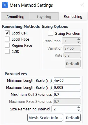
Simulation Setup:
The simulation consists of the 2D gearbox with 2 gears in it. Transient dynamic simulation is performed with VoF method. The rotational velocity of 2.0e2 rad/sec is given to both the gears (opp direction). k-epsilon realizable turbulence model is used in the framework of Navier-stokes equations. The second-order cell-centered finite volume method is used to discretize the differential equations. SIMPLE algorithm is used for pressure velocity coupling.
We will be using the Smoothing and Remeshing method for dynamic mesh simulation.

Primary Fluid = Air

Secondary Fluid = Oil/n-heptane

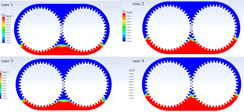
Case 1: 20% Immersion, Fluid - Engine Oil

Case 2: 30% Immersion, Fluid - Engine Oil

Case 3: 20% Immersion, Fluid-n-heptane (c7h16)

Case 4: 30% Immersion, Fluid-n-heptane (c7h16)

i) Engine Oil

Density = 870 kg/m3

Viscosity = 0.174 kg/m-s

ii) n-heptane (c7h16)

Density = 684 kg/m3

Viscosity = 0.000409 kg/m-s

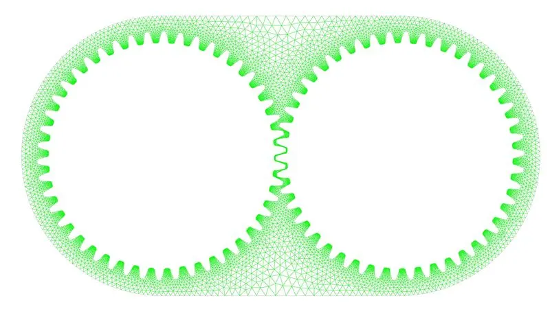
Initial Mesh:

Origin is located at the center of the left gear.

UDF:

#include "udf.h"

DEFINE_CG_MOTION(right_motion, dt, vel, omega, time, dtime)
{
	vel[0] = 0.0;
	vel[1] = 0.0;
	vel[2] = 0.0;

	omega[0] = 0.0;
	omega[1] = 0.0;
	omega[2] = 2.0e2; /* [rad/s]*/
}
DEFINE_CG_MOTION(left_motion, dt, vel, omega, time, dtime)
{
	vel[0] = 0.0;
	vel[1] = 0.0;
	vel[2] = 0.0;

	omega[0] = 0.0;
	omega[1] = 0.0;
	omega[2] = -2.0e2; /* [rad/s]*/
}

Time Step of all the cases = 0.0001sec

Number of Time Steps = 400-500\

Results:

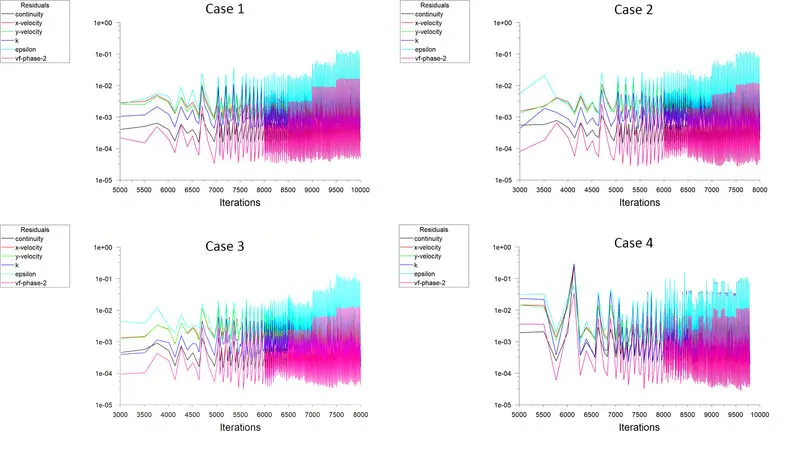
Conclusion:

It has been observed in the simulation that the case with 30% filled oil/secondary_fluid wets the gear more than in 20% case of both the fluid used. The oil/secondary_fluid is getting more trapped in the gear tooth in the 30% case of both types of fluids used which will lubricate the gear properly.

The viscosity of Engine Oil is higher than n-heptane due to which Oil is trapped in the gear tooth for more time.