Week 8 - Simulating Cyclone separator with Discrete Phase Modelling

WEEK 8 - SIMULATING CYCLONE SEPARATOR WITH DISCRETE PHASE MODELLING

AIM:

• To write a few words about any four empirical models used to calculate the cyclone separator efficiency.
• To perform an analysis on a given cyclone separator model by varying the particle diameter from 1 μm to 5 μm and calculate the separation efficiency in each case by keeping velocity constant as 3 m/s. Discuss the results.
• To perform an analysis on a given cyclone separator model by varying the particle velocity from 1 m/sec to 5 m/sec and calculate the separation efficiency and pressure drop in each case by keeping the particle diameter constant as 5 μm.
• Discuss the results.

Theory:

IOZIA AND LEITH MODEL:

• Iozia and Leith (1990) logistic model is a modified version of Barth (1956) model which is developed based on force balance.
• The model assumes that a particle carried by the vortex endures the influence of two forces: a centrifugal force, Z, and a flow resistance, W.
• Core length, zc, and core diameter, dc, are given as

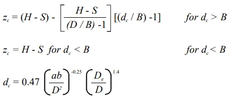
• The addition made by Iozia and Leith on the original Barth (1956) model are the core length zc and slope parameter β expression which is derived based on the statistical analysis of experimental data of cyclone with D = 0.25 m.
• The collection efficiency ηi of particle diameter dpi can be calculated from

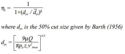
LI AND WANG MODEL:

• The Li and Wang (1989) model includes particle bounce or re-entrainment and turbulent diffusion at the cyclone wall. A
  two-dimensional analytical expression of particle distribution in the cyclone is obtained.
• Li and Wang model was developed based on the following assumptions:

1. The radial particle velocity and the radial concentration profile are not constant, for uncollected particles within the
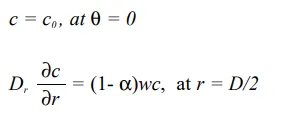
   cyclones.
2. Boundary conditions with the consideration of turbulent diffusion coefficient and particle bounce re-entrainment on
   the cyclone wall are:

3. The tangential velocity is related to the radius of cyclone by:
uRn = constant.

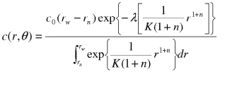
The concentration distribution in a cyclone is given as:

where,

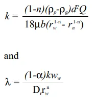
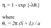
4. The resultant expression of the collection efficiency for particle
of my size is given as

KOCH AND LICHT MODEL:

1. Koch and Licht (1977) collection theory recognized the inherently turbulent nature of cyclones and the distribution of
   gas residence times within the cyclone.
2. Koch and Licht describe particle motion in the entry and collection regions
   with the additional following assumptions:

• The tangential velocity of a particle is equal to the tangential velocity of the gas flow, i.e. there is no slip in the tangential
  direction between the particle and the gas.
• The tangential velocity is related to the radius of cyclone by:
  uRn = constant.

A force balance and an equation on the particles collection yields the grade efficiency ηi.

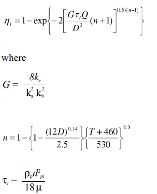
G is a factor related to the configuration of the cyclone, n is related to the vortex and τ is the relaxation term.

LAPPLE MODEL:

• Lapple (1951) model was developed based on force balance without considering the flow resistance. Lapple assumed that a particle entering the cyclone is evenly distributed across theinlet opening.
• The particle that travels from inlet half width to the wall in the cyclone is collected with 50% efficiency.
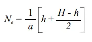
• The semi empirical relationship developed by Lapple (1951) to calculate a 50% cut diameter, dpc, is

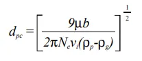
where Ne, is the number of revolutions

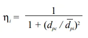
The efficiency of collection of any size of particle is given by

Procedure:

1. Spaceclaim:

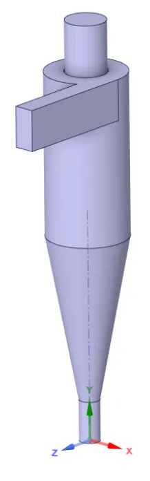
• Firstly, we need to open the spaceclaim and import the given geometry.
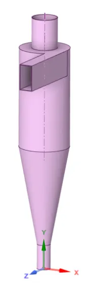
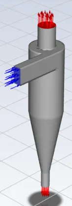
• Now we need to extract the volume by using the edge tool in the volume extract option by selecting the edges of two outlets and one inlet.
• Now we need to suppress the cyclone separator not the volume extracted geometry.
• Close Spaceclaim.

2. Meshing:

• Firstly we need to open the mesh in the workbench.
• Now we need to do generate the baseline mesh and see to get the basic idea.
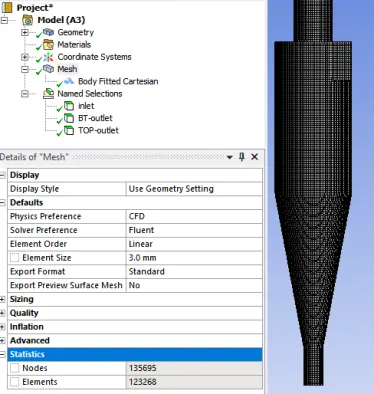
• Now we can refine the mesh and here body fitted catresian mesh is used which is done by inserting the method and select cartesian from the settings, since it is a tapered geometry so the genetated mesh will not be uniform structured throughout the geometry.
• Update the mesh and close it.

3. Set-up:

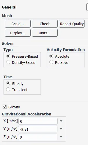
• Firstly we need to choose the steady and gravity options for this analysis.

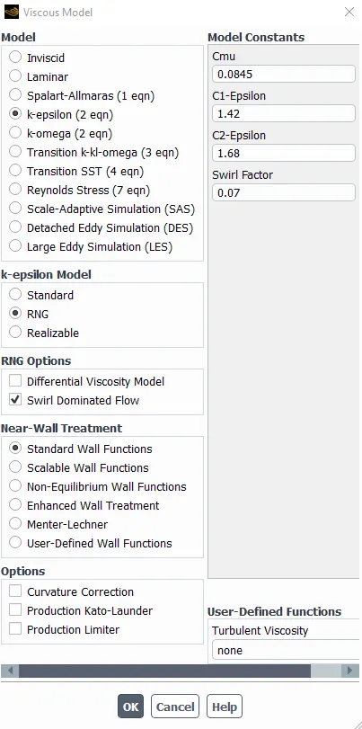
• Now we need to select the viscous model as K-epsilon, RNG, swirl dominant and standard wall functions.

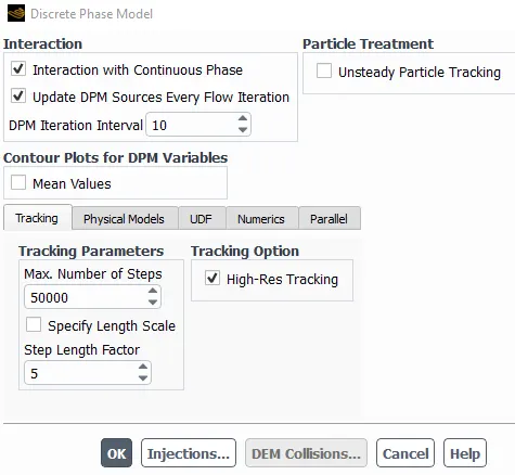
• Now we need to enable discrete phase modelling and select "interaction with continuous phase" and "update DPM sources every flow iteration".

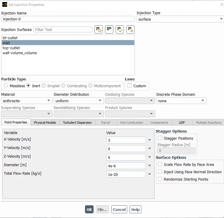
• Now we need to create injections and set particle type as inert, material anthracite, injection type surface, in injection propeties compute from inlet and give the value for velocity and also for particle diameter.

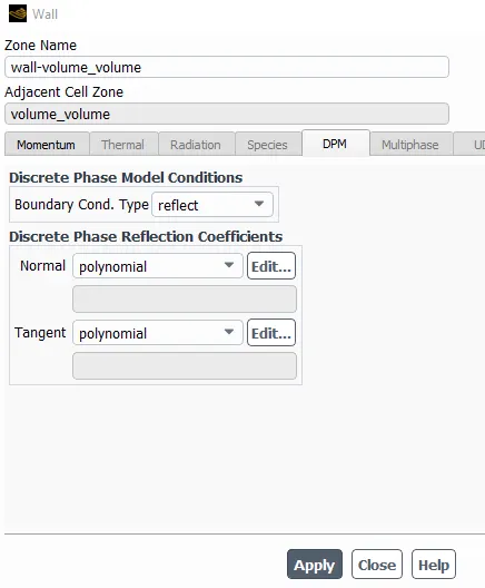
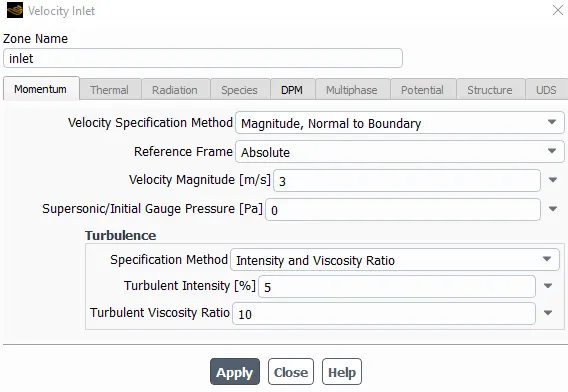
• Set the boundary conditions as follows;

1. Inlet reflect, give the value for velocity
2. wall reflect
3. bottom outlet trap
4. top outlet escape.

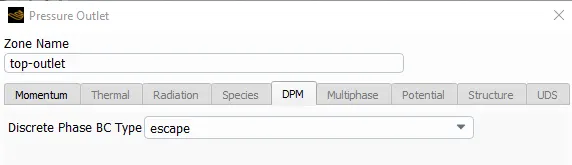
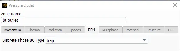
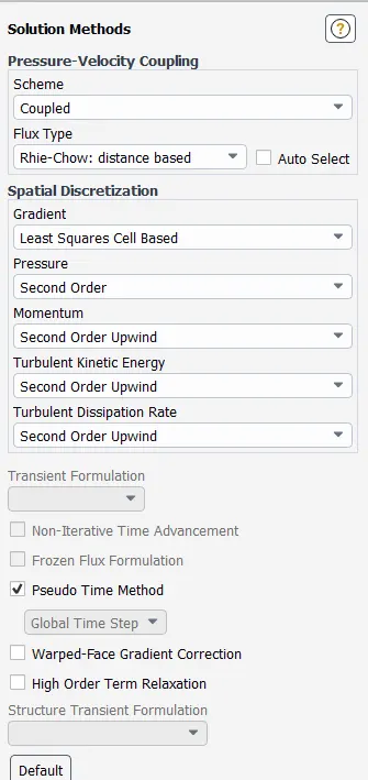
• In methods, select the turbulent kinetic energy and turbulent dissipation rate as second order upwind.

• We can use hybrid or standard initialisation but here it is initialised by standard.
• We also need to have particle tracking data and this data has to be exported so that it can be saved in our folder and later when it is required it can be imported to the CFD post.

4. Results:

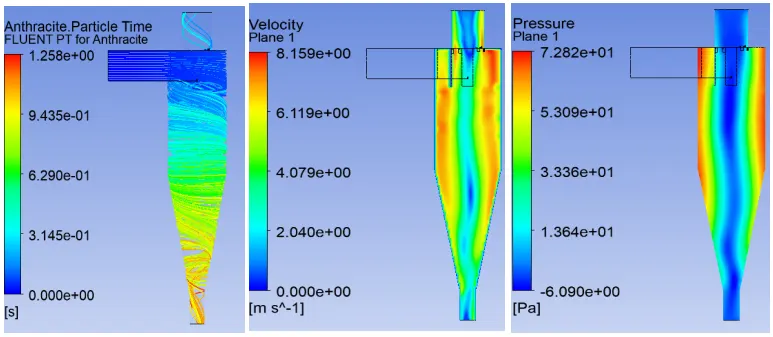
Particle diameter constant with value 5e-6 μm by varying velocity from 1 m/s to 5 m/s:

case-1; 1 m/s, 5 μm:

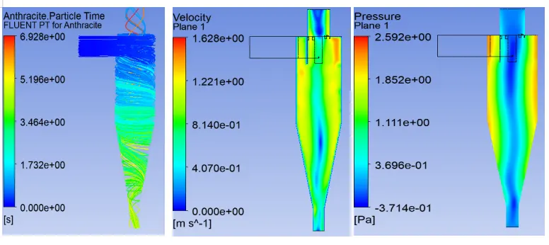
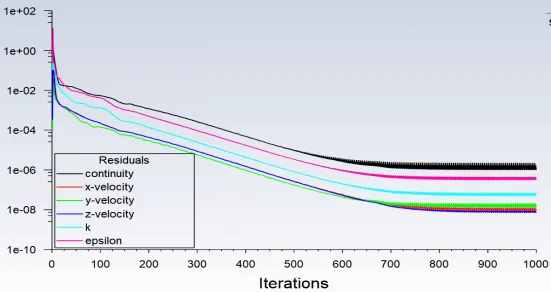
case-2; 3 m/s, 5 μm:

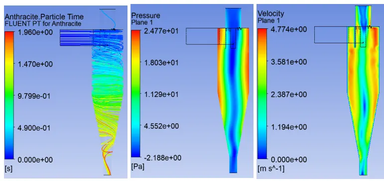
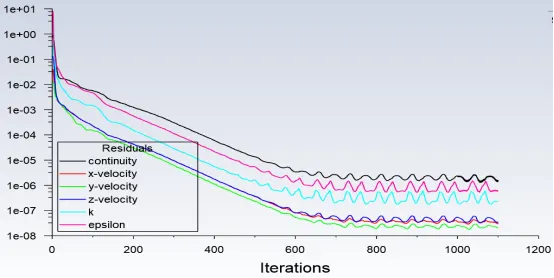
case-3; 5 m/s, 5 μm:

Animation link:

https://drive.google.com/file/d/1QJjxX6dl_12bmZIl1jWAOPSdxJu2B1PR/view?usp=sharing

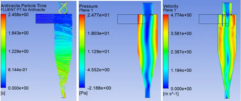
Velocity constant with value 3 m/s by varying particle diameter from 1 μm to 5 μm:

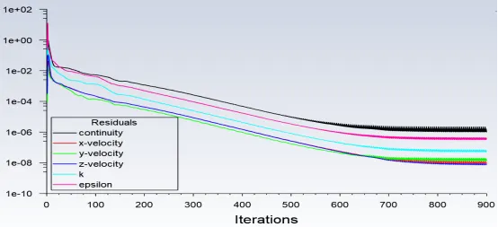
case-1; 1 μm, 3 m/s:

Animation link:

https://drive.google.com/file/d/1pk4qGfOWKoIpfilcvQXP2r_tTjxnatp-/view?usp=sharing

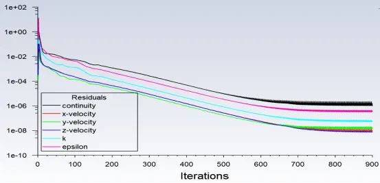
case-2; 2.5 μm, 3 m/s:

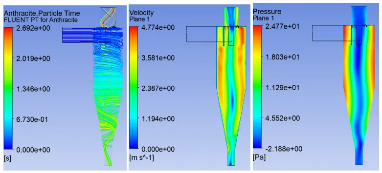
Animation link:

https://drive.google.com/file/d/1qMQtv5uTg6EcOnlp5mUYyohtFtUiXBb9/view?usp=sharing

case-3; 4 μm, 3 m/s:

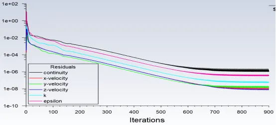
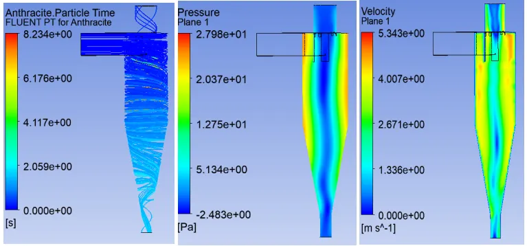
Animation link:

https://drive.google.com/file/d/1aC21TAEbzfe7jdKjKtpIwDSx6TDVLAeF/view?usp=sharing

Conclusion:

Tabulation:

Particle diameter constant with value 5e-6 μm by varying velocity from 1 m/s to 5 m/s:

Particle Velocity (m/s)	Particle diameter (μm)	No of patricles tracked	No of particles trapped	No of particles escaped	Separator efficiency (%)	pressure drop (Pa)
1	5	180	149	28	82.77	39.732
3	5	180	156	17	86.66	26.958
5	5	180	157	23	87.72	78.918

• The higher the velocity of the particle, separator efficiency increases and this is because increase in number of trapped particles, when the velocity increases.
• The higher the velocity of the particle, pressure drop also increases in cyclone separator.

Velocity constant with value 3 m/s by varying particle diameter from 1 μm to 5 μm:

Particle Velocity (m/s)	Particle diameter (μm)	No of patricles tracked	No of particles trapped	No of particles escaped	Separator efficiency (%)	pressure drop (Pa)
3	1	180	135	23	75	15.958
3	2.5	180	146	45	81.11	26.958
3	4	180	150	27	83.33	30.463

• The higher the value of the diameter particle, separator efficiency increases and this is because increase in number of trapped particles, when the particle diameter increases .
• The higher the value of the particle diameter, pressure drop also increases .