Week 8 - Simulating Cyclone separator with Discrete Phase Modelling
Simulating Cyclone separator with Discrete Phase Modelling
Aim:- To perform analysis on cyclone separator and calculate the separation efficiency and pressure drop.
Objective(s):-
- To write a few words about any four empirical models used to calculate the cyclone separator efficiency.
- To perform an analysis on a given cyclone separator model by varying the particle diameter from 1 μm to 5 μm and calculate the separation efficiency in each case. Discuss the results. [Use both the velocity's as 3m/sec.]
- To perform an analysis on a given cyclone separator model by varying the particle velocity from 1 m/sec to 5 m/sec and calculate the separation efficiency and pressure drop in each case. Discuss the results. [Use particle diameter size as 5 μm for all cases & keep flow velocity same as particle velocity].
Theory :
A cyclone separator :
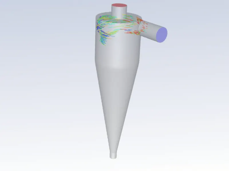
Cyclone separators or simply cyclones are separation devices (dry scrubbers) that use the principle of inertia to remove particulate matter from flue gases. Cyclone separators is one of many air pollution control devices known as precleaners since they generally remove larger pieces of particulate matter. This prevents finer filtration methods from having to deal with large, more abrasive particles later on. In addition, several cyclone separators can operate in parallel, and this system is known as a multicyclone.
Four empirical models to calculate the cyclone separator efficiency :
1. Iozia and Leith Model
Iozia and Leith [4] logistic model is a modified version of Barth Model, which is developed based on force balance.
The model assumes that a particle carried by the vortex endures the influence of two forces: a centrifugal force, Z and a flow resistance, W. The collection efficiency ηi of particle diameter dpi can be calculated from :
`n_i = 1/(1 + ((d_(pc))/(d_(pI)))^beta`
β is an expression for slope parameter derived based on the
statistical analysis of experimental data of a cyclone with D = 170
0.25 m given as `beta = 0.62 - 0.87ln((d_(pc))/100) + 5.21ln((ab)/D^2)+1.05[ln((ab)/(D^2))]`
here dpc is the 50% cut size given by Barth
`d_(pc) = [(9*mu*Q)/(pi*rho*Z_c*v_(tmax)^2)]`
here the core length `Z_c`and the core diameter `d_c`are given as:
`Z_c = (H-S) - [(H-S)/((D/B) - 1)]*[(d_c/B - 1)]` for `d_c >B` or
`Z_c = H-S` for `d_c < B`
`d_c = 0.47D((ab)/D^2)^(-0.25)*((D_e)/(D))`
2. Li and Wang model :
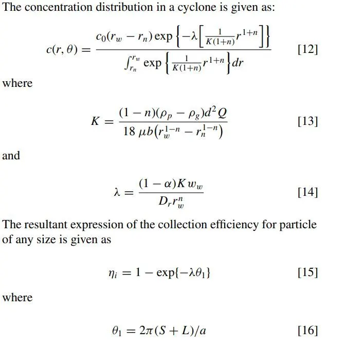
The Li and Wang [3] model includes particle bounce or reentrainment and turbulent diffusion at the cyclone wall. A twodimensional analytical expression of particle distribution in the cyclone is obtained. Li and Wang model was developed based on the following assumptions:
• The radial particle velocity and the radial concentration profile are not constant for uncollected particles within the cyclone.
• Boundary conditions with the consideration of turbu185 lent diffusion coefficient and particle bounce reentrainment on the cyclone wall are:
1. c = c0, at θ = 0
2. `D_r*((delc)/(delr)) = (1-alpha)*omegac`, at r = D/2.
The tangential velocity is related to the radius of the cyclone by : `uR^n` = constant.
3. Koch and Licht Model :
Koch and Licht collection theory recognized the inherently turbulent nature of cyclones and the distribution of gas residence times within the cyclone. Koch and Licht described particle motion in the entry and collection regions with the additional following assumptions:
• The tangential velocity of a particle is equal to the tangential velocity of the gas flow, i.e. there is no slip in the tangential direction between the particle and the gas.
• The tangential velocity is related to the radius of cyclone by: u Rn = constant.
A force balance and an equation on the particles collection yields the grade efficiency ηi
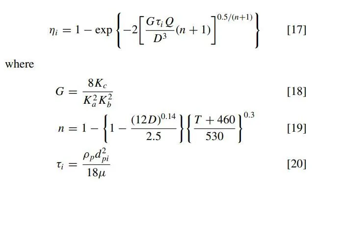
G is a factor related to the configuration of the cyclone, n is related to the vortex and τ is the relaxation term.
4. Lapple model :
Lapple [1] model was developed based on force balance without considering the flow resistance. Lapple assumed that a particle entering the cyclone is evenly distributed across the inlet opening. The particle that travels from inlet half width to the wall in the cyclone is collected with 50% efficiency. The semiempirical relationship developed by Lapple to calculate a 50% cut diameter, dpc, is
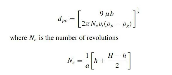
The efficiency of collection of any size of particle is given by
`eta = 1/(1+((d_(pc))/(d_(pI)))^2`
General formula for calculating the efficiency of the cyclone separator :
`eta_(cyclo) =`(number of the particles trapped)/(number of the particles tracked).
Modelling and simulation approach :
Modelling in SpaceClaim :
1.Launch the ANSYS Workbench and double click on the FLUENT analysis system. Then double click on the SpaceClaim component to launch it.
2.Import the cyclone separator geometry file into the SpaceClaim.
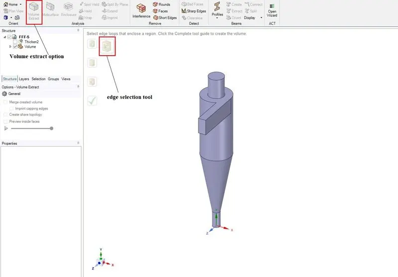
3. Extract the fluid volume using the prepare option. Supress the solid geometry for physics.
4. Exit the spaceClaim
Meshing :
1.Launch the ANSYS Mesher and the software should automatically attach the geometry.
2.Navigate to the "Mesh" option in the tree and click on it. Now navigate to the Mesh options which appear as a window below it.
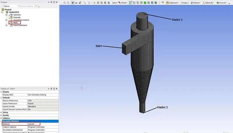
3. Choose the "cutcell" method in the assembly meshing. Now select the appropriate faces and name them as inlet, outlet 1 and outlet 2.
4. Change the element size to 10mm and click on generate mesh.
Setting up the case in ANSYS FLUENT :
1. launch the FLUENT.
2. In the General tab click on the gravity option and input the value of -9.81 m/s^2 in the text field.
3. In the turbulence models, select the K-epsilon RNG with swirl dominated flow option.
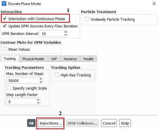
4. In order to enable the Discrete Phase Modelling, double click on the Discrete phase icon in the models section. A window pops up which looks like the above image.
5. Check the Interaction with the continuous phase option which enables the other option Update DPM sources every flow iteration. Check that option too and set the DPM iteration interval as 10. Proceed with the default values of the for the Tracking parameters.
6. The important part in Discrete phase modelling is defining the dispersed phase. In order to do that click on the injections and another pop up window opens.
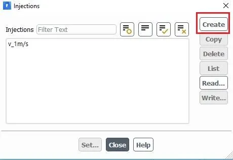
7. In the window titled Injections, click on the create button and it should open another pop up window in which we define the properties of the dispersed phase.
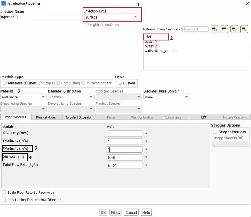
8. As shown in the above figure, set the injection type to surface and release injections from surface to inlet. Also in the variables section, change the velocity of the particle in accordance with the case (1 m/s or 2 m/s ......or 5 m/s) and diameter as 1e-6 or 2e-6.......or 5e-6.
9. Click on OK and navigate to the boundary conditions tab.
10. For the inlet, input the velocity according to the case and in the DPM tab change Discrete phase boundary condition type to reflect.
11. For the boundaries like outlets and walls the Discrete phase boundary condition is set as follows by default which are correct.
Boundary Conditions:-
Outlet(Top):- Escape
Outlet(Bottom/dustbin) - Trap
12.Initialize the solution using the standard method with the values available from the inlet.
13. Run the simulation for 1000 iterations and export the particle histrory data.
Results :
Setup.I : Constant velocity of 3m/s and varying particle velocity
a. Particle diameter of 1e-6 m
i. Pressure contour plot ii. Velocity contour plot
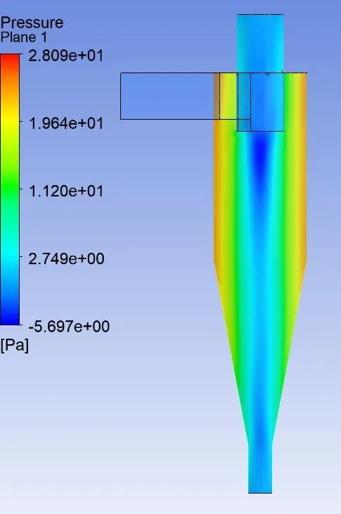
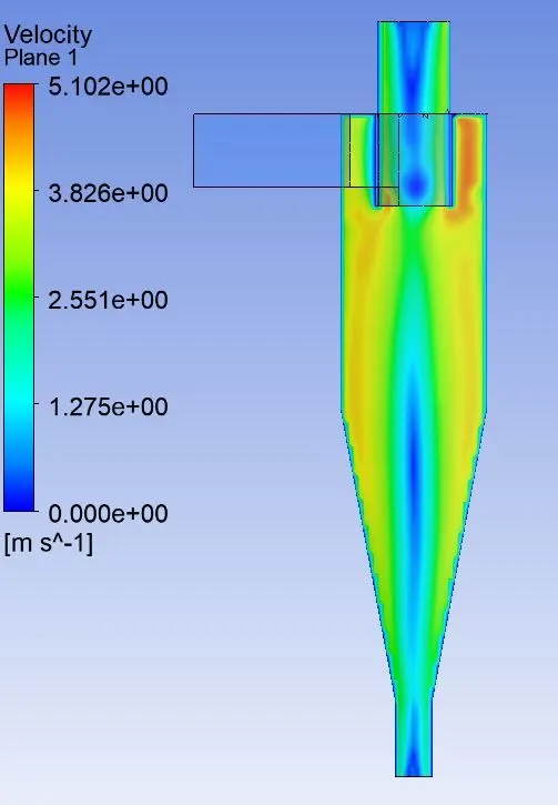
iii. Particle time inside the cyclone separator iv. vortex strength contour
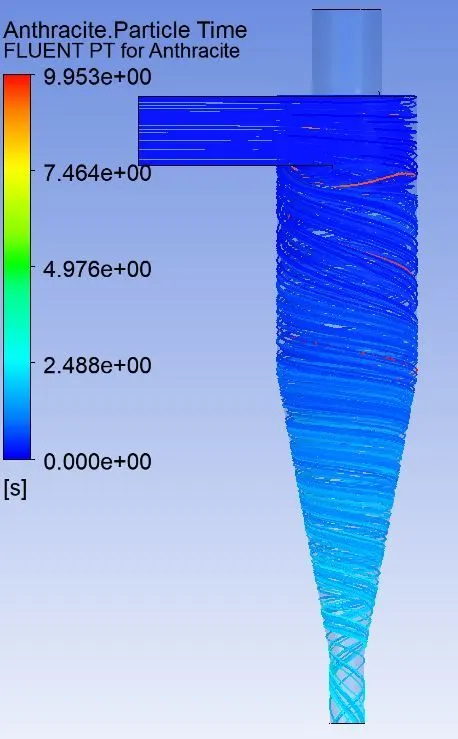
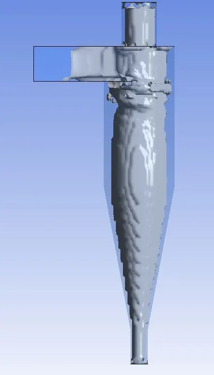
Animation file for the Particle motion inside the cyclone separator:
b. Particle diameter of 2e-6 m
i. Pressure contour ii. Velocity contour
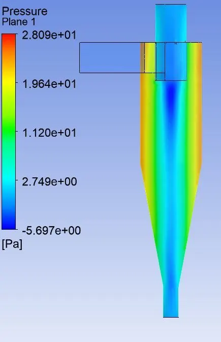
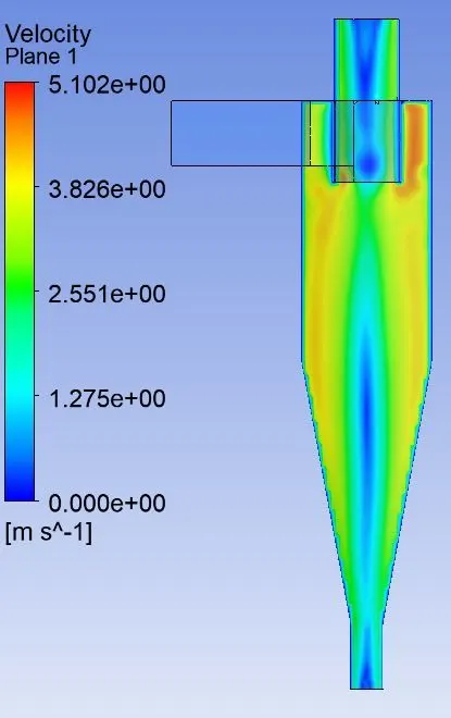
iii. Particle time spent in the cyclone separator iv. Vortex strength contour
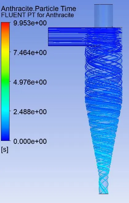
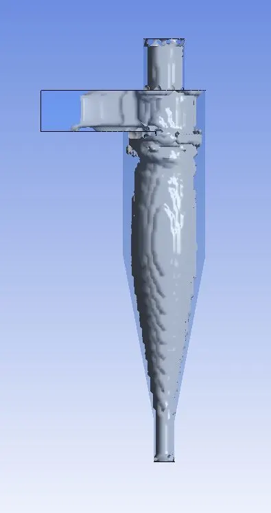
v. Animation file for the particle motion inside the cyclone separator :
c. Particle diameter of 3e-6
i. Pressure contour ii. Velocity contour
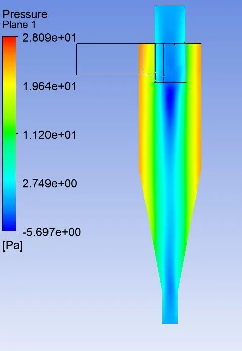
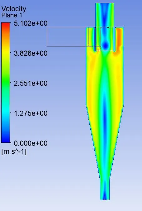
iii. Particle time inside the cyclone separator iv. Vortex strength
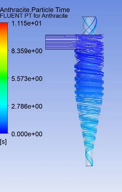
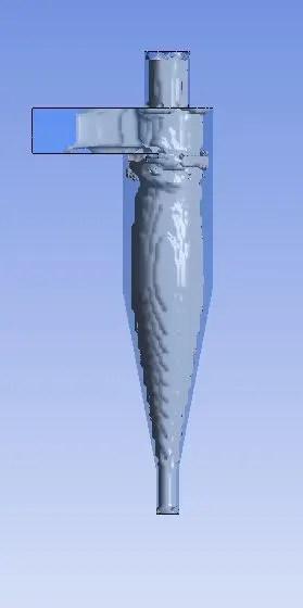
v. Animation file of the particle motion inside the cyclone separator.
d. Particle diameter of 4e-6
i. Pressure contour ii. Velocity contour
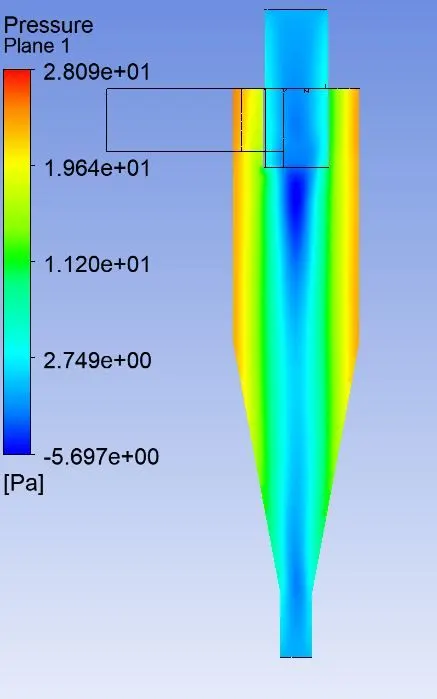
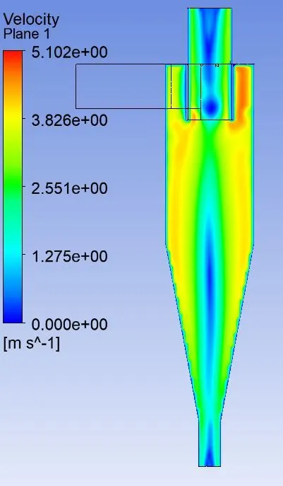
iii. Particle time inside the cyclone separator iv. Vortex strength
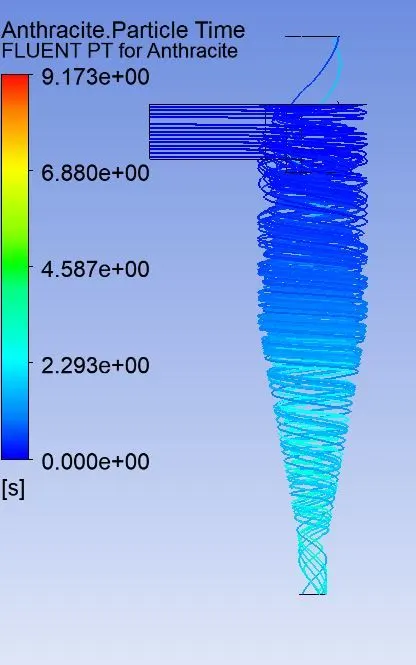
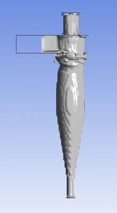
v. Animation file of the particle motion inside the cyclone separator
e. Particle diameter of 5e-6
i. Pressure contour ii. Velocity contour
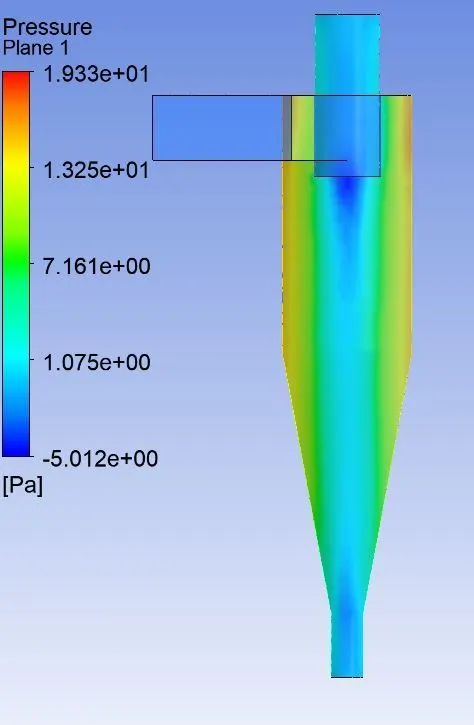
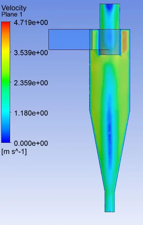
iii. Particle time inside the cyclone separator iv. Vortex strength
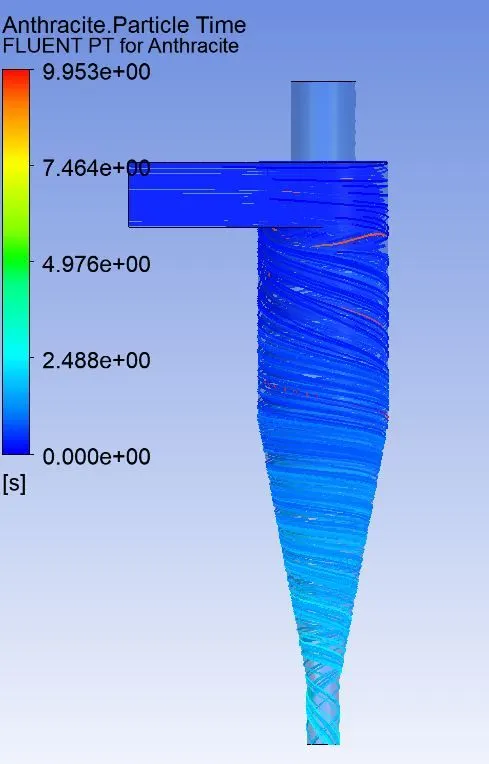
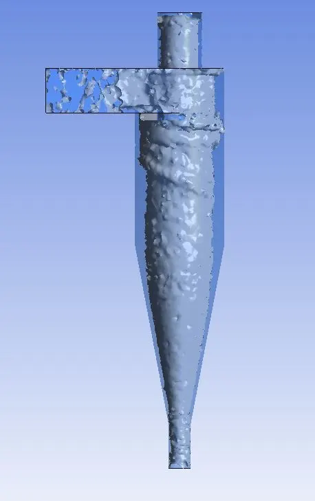
v. Animation file of the particle motion inside the cyclone separator
Setup.2 : Constant particle size of 5`mu m`and varying particle velocity
1. Particle velocity of 1 m/s
i. Pressure contour ii. Velocity contour
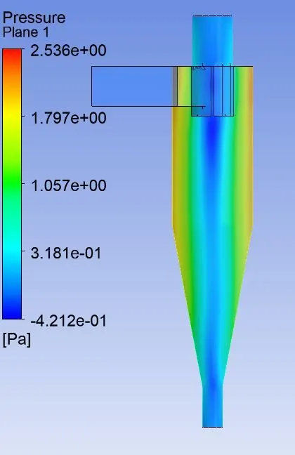
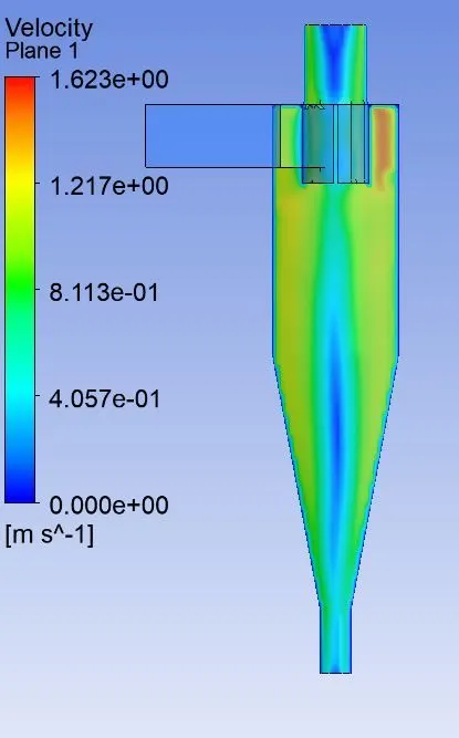
iii. Particle time inside the cyclone separator iv. Vortex strength
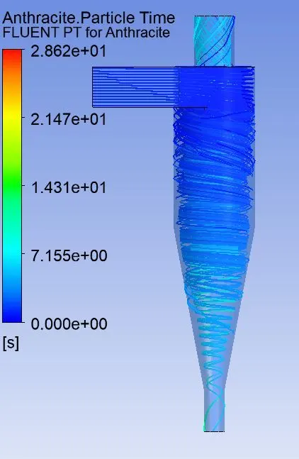
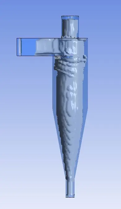
v. Animation file of the particle motion inside the cyclone separator
2. particle velocity of 2 m/s
i. Pressure contour ii. Velocity contour
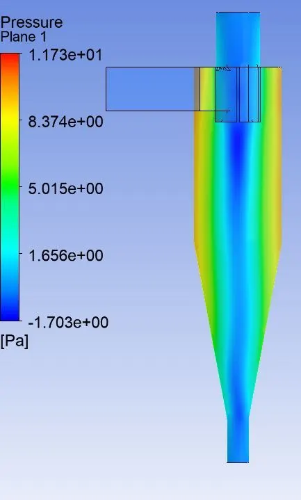
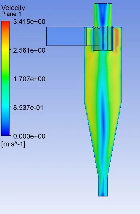
iii. Particle time inside the cyclone separator iv. Vortex strength
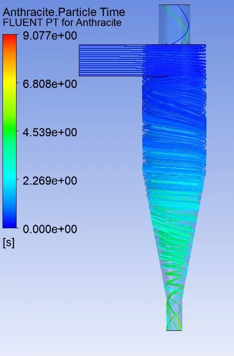
v. animation of the particle motion inside the cyclone separator
3. particle velocity of 3 m/s
i. Pressure contour ii. Velocity contour
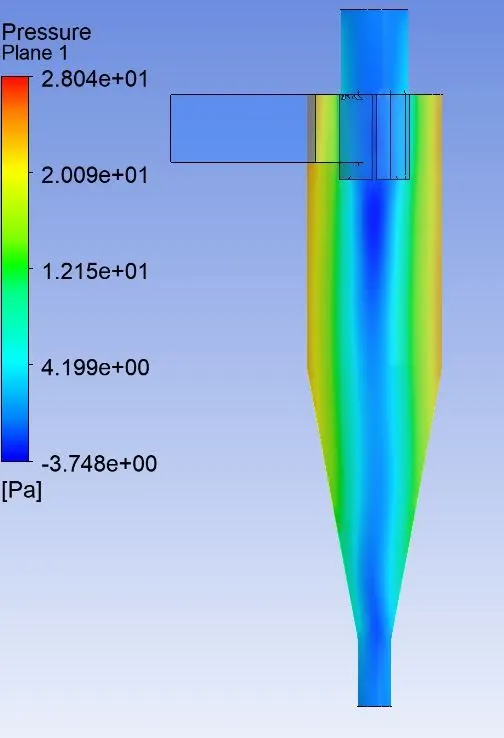
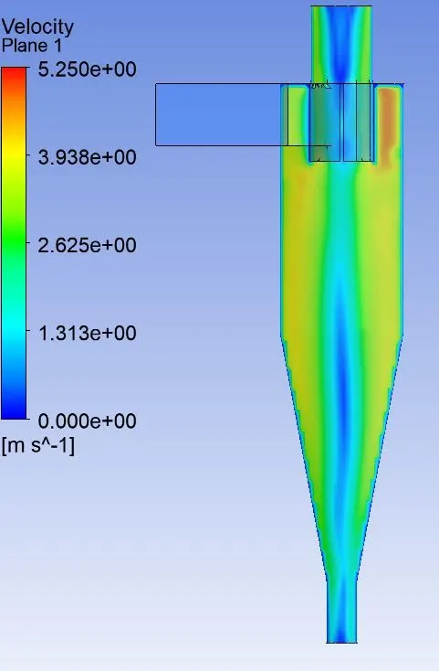
iii. Particle time spent in the cyclone separator iv. Vortex strength
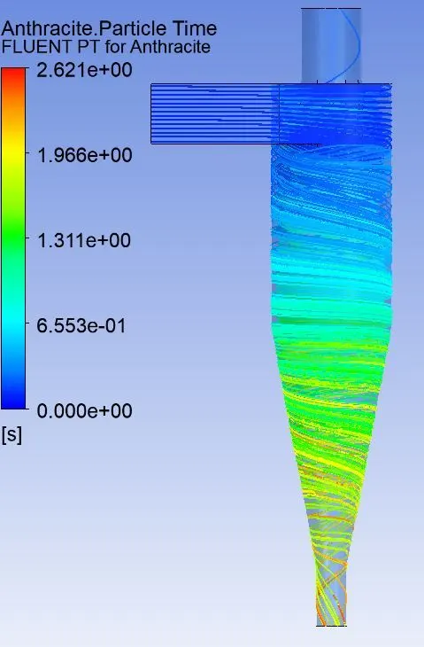
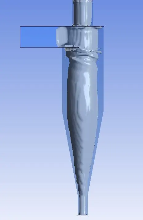
v. Animation file of the particle motion inside the cyclone separator
4. Particle velocity of 1m/s
i. Pressure contour ii. Velocity contour
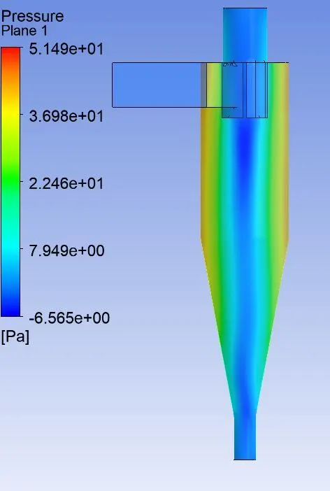
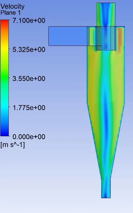
iii. Particle time inside the cyclone separator iv. Vortex strength
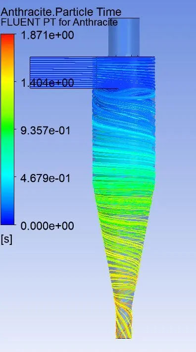
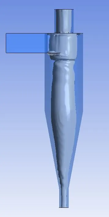
v. Animation file of the particle motion inside the cyclone separator
5. Particle velocity of 5 m/s
i. Pressure contour ii. Velocity contour
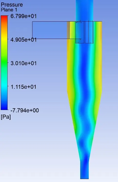
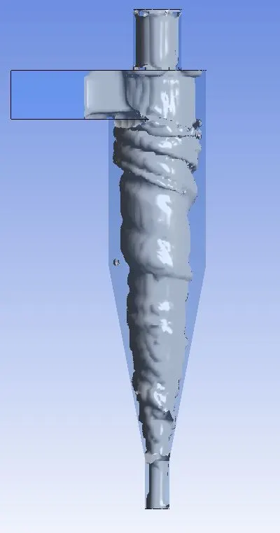
v. Animation file of the particle motion inside the cyclone separator
Tabular form of the results :
| Velocity of the particle | Inlet pressure | Outlet pressure 1 | Outlet pressure 2 |
pressure difference (`DeltaP`) = `P_(i) - P_(o1)` |
Efficiency of the cyclobne separator(`eta`) |
| 1 m/s | 2.455 Pa | -8.6e-4 Pa | -4.64e-5 Pa | 2.45586 Pa | |
| 2 m/s | 11.268 Pa | -64.73e-4 Pa | -20.4e-4 Pa | 11.2744 Pa | |
| 3 m/s | 26.28 Pa | -18.3e-3 Pa | -7.8e-3 Pa | 26.298 Pa | |
| 4 m/s | 49.220 Pa | -3.6e-2 Pa | -17.9e-3 Pa | 49.256 Pa | |
| 5 m/s | 64.423 Pa | -6.69e-2 Pa | - 5.6e-4 Pa | 64.4899 Pa |
Calculation of efficiency of the cyclone separator :
case.1 : constant velocity of 3m/s and variable particle size
| Particle diameter | No. of partcles tracked | No.of Particles escaped | No. of particles trapped | No.of particles incomplete | Separation efficiency(`eta`) |
| 1e-6 | 435 | 213 | 218 | 4 | 50.11 |
| 2e-6 | 435 | 198 | 236 | 1 | 54.2 |
| 3e-6 | 435 | 182 | 253 | 0 | 58.16 |
| 4e-6 | 435 | 149 | 286 | 0 | 65.74 |
| 5e-6 | 435 | 109 | 326 | 0 | 74.94 |
case.2 : Varying velocity and constant particle size of 1e-6m
| Velocity(in m/s) | Particle diameter in m | Separation efficiency(`eta`) |
| 1 | 5e-6 | 25.2% |
| 3 | 5e-6 | 69.8% |
| 5 | 5e-6 | 89.7% |
Result analysis :
1. Higher the particle diameter, higher is the separation efficiency of the cyclone separator.
2. Increase in particle speed also increases the separtion efficiency of the cyclone separator.
3. It can be said that the given cyclone separator works best with the particles of higher diameter.
Conclusion :
A CFD simulation on the working of the cyclone separator in performed and based on the simultion results, the separation efficiency is determined.
References:
1. Theory of cyclone separtors : https://energyeducation.ca/encyclopedia/Cyclone_separator.
2. Empirical models for calulation of the separator efficiency : https://www.researchgate.net/publication/232747389_A_CFD_Study_on_the_Prediction_of_Cyclone_Collection_Efficiency