Week 8 - Simulating Cyclone separator with Discrete Phase Modelling
Cyclonic separator
Cyclonic separation:-
Cyclonic separation is a method of removing particulates from an air, gas, or liquid stream, without the use of filters, through vortex separation. Rotational effects and gravity are used to separate mixtures of solids and fluids.
Cyclonic separator:-
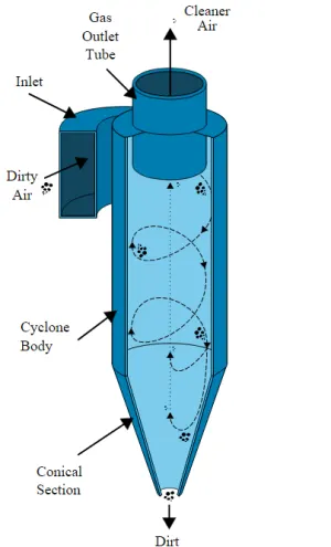
A high-speed rotating (air)flow is established within a cylindrical or conical container called a cyclone. Air flows in a helical pattern, beginning at the top (wide end) of the cyclone and ending at the bottom (narrow) end before exiting the cyclone in a straight stream through the center of the cyclone and out the top. Larger (denser) particles in the rotating stream have too much inertia to follow the tight curve of the stream, and thus strike the outside wall, then fall to the bottom of the cyclone where they can be removed. In a conical system, as the rotating flow moves towards the narrow end of the cyclone, the rotational radius of the stream is reduced, thus separating smaller and smaller particles. The cyclone geometry, together with the volumetric flow rate, defines the cut point of the cyclone. This is the size of particle that will be removed from the stream with a 50% efficiency. Particles larger than the cut point will be removed with greater efficiency and smaller particles with a lower efficiency as they separate with more difficulty or can be subject to re-entrainment when the air vortex reverses direction to move in direction of the outlet.
Cyclone separator working:-
Cyclone separators work much like a centrifuge, but with a continuous feed of dirty air. In a cyclone separator, dirty flue gas is fed into a chamber. The inside of the chamber creates a spiral vortex, similar to a tornado. The lighter components of this gas have less inertia, so it is easier for them to be influenced by the vortex and travel up it. Contrarily, larger components of particulate matter have more inertia and are not as easily influenced by the vortex.
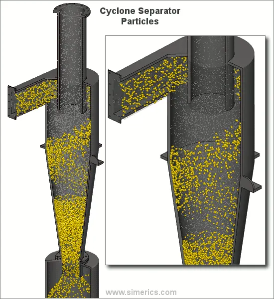
Since these larger particles have difficulty following the high-speed spiral motion of the gas and the vortex, the particles hit the inside walls of the container and drop down into a collection hopper. These chambers are shaped like an upside-down cone to promote the collection of these particles at the bottom of the container. The cleaned flue gas escapes out the top of the chamber.
Most cyclones are built to control and remove particulate matter that is larger than 10 micrometers in diameter. However, there do exist high-efficiency cyclones that are designed to be effective on particles as small as 2.5 micrometers. As well, these separators are not effective on extremely large particulate matter. For particulates around 200 micrometers in size, gravity settling chambers or momentum separators are a better option.
Out of all of the particulate-control devices, cyclone separators are among the least expensive. They are often used as a pre-treatment before the flue gas enters more effective pollution control devices. Therefore, cyclone separators can be seen as "rough separators" before the flue gas reaches the fine filtration stages.
Cyclone separators are actually able to remove this matter depending largely on particle size. If there is a large amount of lighter particulate matter, fewer of these particles are able to be separated out. Because of this, cyclone separators work best on flue gases that contain large amounts of big particulate matter.
Advantages:-
- These cyclone separators are beneficial because they are not expensive to install or maintain
- They don't have any moving parts i.e, maintenance and operating costs are low.
- The removed particulate matter is collected when dry, which makes it easier to dispose of.
- These units take up very little space.
Disadvantages:-
- Because of standard models are not able to collect particulate matter that is smaller than 10 micrometers effectively.
- These machines are unable to handle sticky or tacky materials.
Applications:-
- Some cyclone models are predesigned for specific applications, while others are built for specialized environments.
- Among the most important application considerations is the dust and gas composition.
- Specific types of particulate may be corrosive, abrasive, sticky, explosive, or toxic, thus requiring special construction materials or designs in order to function properly.
- Cyclones are used for filtration of abrasives, coolant mists, explosive media, fine powders, metalworking chips, toxic media, and various production plant exhausts.
Specifications:-
-
Airflow or volumetric flow rate:-
-
volumetric flow rate is the airflow generated or handled by a cyclone. This is usually given in cubic feet per minute (cfm). Some manufacturers provide ranges in standard cubic feet per minute (scfm), as flow rates can vary greatly as environmental conditions stray for standard temperature and pressure. To convert a given actual flow rate (QA) in actual cubic feet per minute (acfm) to standard flow (QS) in scfm, utilize the combined ideal gas equation.
-
which includes volume (V), pressure (P), and temperature (T) at actual and standard conditions.
-
`(P_S*V_S)/T_S = (P_A*V_A)/T_A`
-
If we know the temperature and pressure at actual conditions, we can substitute volume (V) with flow rate (Q, equivalent to volume per unit time) and rearrange to solve for QS.
-
`Q_S = Q_A • (P_A/P_S) • (T_S/T_A)`
-
A cyclone with a higher airflow can accommodate larger gas streams for treatment. For effective operation, the airflow of the system at the point of installation should fall within the rated airflow range of the cyclone.
-
-
Minimum filtered particle size
-
Minimum filtered particle size is the smallest particle size a cyclone can filter. It is generally measured in microns or micrometers (µm).
-
-
Separation or Collection efficiency:-
-
Separation efficiency, capture rate, or recovery rate is the overall removal efficiency of Particulate matter from an air stream. Manufacturers sometimes provide estimated efficiencies upfront; however actual results will vary based on the properties of particles in the gas stream, and on certain environmental conditions.
-
-
Pressure drop:-
-
Pressure drop is the amount of flow resistance the cyclone will create in the system. Pressure drop is usually measured in units of inches of water column (in WC) or Pascals (Pa).
-
----------------------------------------------------------------------------------------------------------------------
Four empirical models were used to calculate the cyclone separator efficiency.
1. Iozia and Leith Model
- `eta_i=1/(1 + (d_(pc)/d_(text(pi))))^β`
- β is an expression for slope parameter derived based on the statistical analysis of experimental data of a cyclone with D =0.25 m given as
- `beta = 0.62 − 0.87* ln(d_(pc)/100)+ 5.21* ln((ab)/D^2)+ 1.05*[ln((ab)/D^2)]^2`
- and `d_(pc)` is the 50% cut size given by Barth `d_(pc)=[(9 µQ)/(pi*rho*p^z*c*v_(t max)^2)]^0.5`
- where core length, `z_c`, and core diameter, `d_c`, are given as
- `z_c= (H − S) −[(H − S)/((D/B) − 1)][(d_c/B) − 1] text(for) d_c> B`
- `z_c= H − S text(for) d_c< B`
- `d_c=0.47*D*((ab)/D^2)^-0.25*(D_e/D)^1.4`
- The radial particle velocity and the radial concentration profile are not constant for uncollected particles within the cyclone.
- Boundary conditions with the consideration of turbulent diffusion coefficient and particle bounce re-entrainment on the cyclone wall are:
- `c = c_0,` at `theta = 0`
- `D_r*(delc)/(delr)= (1 − alpha)*wc, text( at ) r = D/2`
- The tangential velocity is related to the radius of the cyclone by`u*R^n= text(constant)`.
- The concentration distribution in a cyclone is given as:
- `c(r, θ) =(c_0*(r_w− r_n)* exp{−lambda[1/(K*(1+n))*r^(1+n)]})/(int_(r_n)^(r_w)exp{1/(K*(1+n))*r^(1+n)}*dr)`
- where `K =((1 − n)(rho_p− rho_g)*d^2*Q)/(18* mu*b(r_w^(1−n)− r_n^(1−n))`
- and `lambda =((1 − alpha)K*w_w)/(D_r*r_w^n)`
-
The resultant expression of the collection efficiency for particle of any size is given as
- `eta_i= 1 − exp{−lambda*theta_1}`
- Where `theta_1= 2pi* ((S + L)/a)`
- The concentration distribution in a cyclone is given as:
- The tangential velocity of a particle is equal to the tangential velocity of the gas flow, i.e. there is no slip in the tangential direction between the particle and the gas.
- The tangential velocity is related to the radius of cyclone by: `u*R^n= text(constant)`
- A force balance and an equation on the particles collection yields the grade efficiency `eta_i`
- `eta_i= 1 − exp{−2[(G*tau_i*Q)/D^3*(n + 1)]^(0.5/(n+1))}`
- where
- `G =(8*K_c)/(K_a^2*K_b^2)`
- `eta = 1 −{1 −(12*D)^0.14/2.5}*{(T + 460)/530}^0.3`
- `tau_i=(rho_p*d_(text(pi))^2)/(18*mu)`
-
`G`is a factor related to the configuration of the cyclone, `n` is related to the vortex and `tau` is the relaxation term.
- where
- `d_(pc)=[(9*mu.b)/(2*pi*N_e*v_i*(rho_p−rho_g))]^(1/2)`
-
where `N_e` is the number of revolutions
- `N_e=1/a[h +(H-h)/2]`
- The efficiency of collection of any size of particle is given by
- `eta_i=1/(1 + (d_(pc)/d_text(pi))^2`
----------------------------------------------------------------------------------------------------------------------
Discrete Phase Model:-
-
Discrete Phase Model is a subsection to Multiphase flows. A discrete phase model (DPM) is used when the aim is to investigate the behavior of the particles from a Lagrangian view and a discrete perspective. The difference between the Lagrangian and the Eulerian view is that fluid behavior in the Lagrangian view is examined based on particle tracking of a particulate flow; Whereas fluid behavior is considered in the Eulerian view based on the assumption of a finite volume element in the fluid flow path.
-
In Discrete Phase Model, the continuous phase is solved using Navier-Stokes equations. At the same time, the discrete phase is simulated by tracking a large number of particles, bubbles, or droplets passing through the calculated continuous flow field. It should be noted that the discrete phase can exchange momentum, mass, and energy with the continuous phase. This method can be made much simpler by ignoring the interaction of particles (as well as droplets and bubbles) with each other. Of course, this can happen when the discrete phase, even with a large mass, has a much smaller volume (less than 10%) than the continuous phase. After each iteration of the continuous phase calculations, the particle paths (as well as bubbles or droplets) are calculated and determined separately.
Procedure:-
- Geometry preparation
- Meshing
- Setup & Solution
- Results
----------------------------------------------------------------------------------------------------------------------
1. Geometry preparation:
- Open Spaceclaim and import the Cyclone Separator 3-D model.
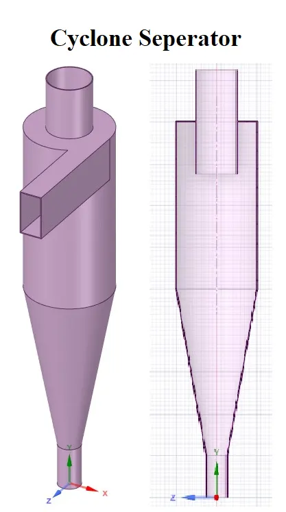
- Use the Volume extract command to extract the Fluid domain.
- Volume extract
- Edge selection(Select boundarys)
- Create volume Enclosure from the selected boundaries
- Fluid domain extracted.
- Create volume Enclosure from the selected boundaries
- Edge selection(Select boundarys)
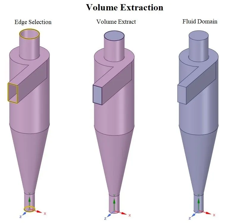
- Hide the Except fluid domain hide all bodies and suppress the for physics.
----------------------------------------------------------------------------------------------------------------------
2. Meshing:
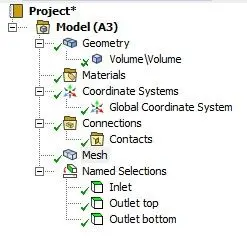
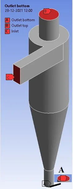
- Create Named sections:-
- Inlet
- Outlet Top
- Outlet Bottom
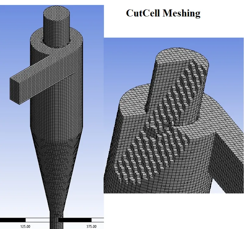
- used CutCell meshing technique for hex-dominant mesh.
- CutCell Meshing:
- Assembly Meshing
- Method = CutCell
- Note:-To enable Assembly Meshing, Open ANSYS Workbench, click Tools > Options > Appearance, select Unsupported Features and click OK
- In sizing max size is given as 10mm while meshing it will automatically adjust the max value.
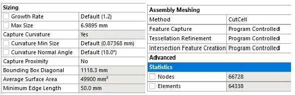
- Assembly Meshing
- CutCell Meshing:
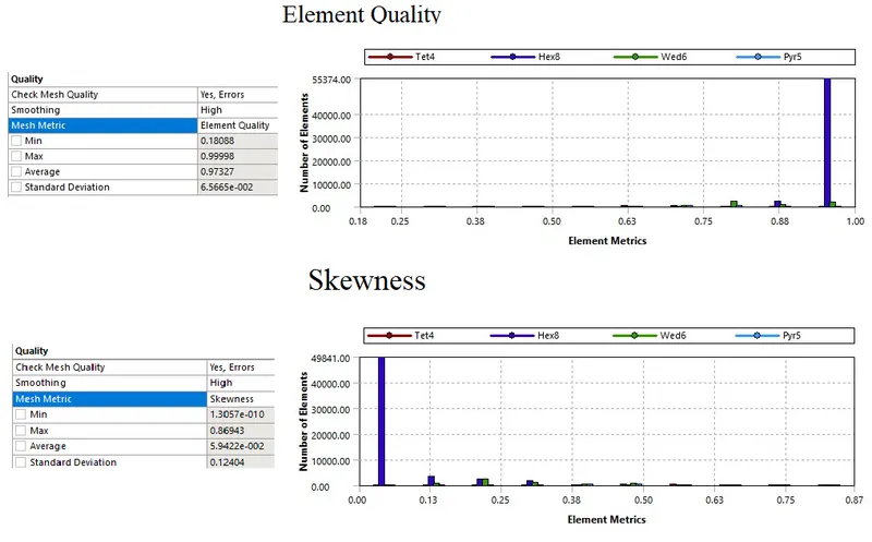
- Mesh:-
- Mesh Quality:-
3. Setup & Solution:-
- Double Precision, Solve processers = 4.
- Solver
- Type = Pressure Based
- Velocity Formulation = Absolute.
- Time= Steady
- Velocity Formulation = Absolute.
- Type = Pressure Based
- Gravity = on
- `Y=−9.81m/s^2`
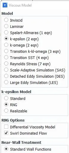
- Viscous model
- k-epsilon
- RNG
- Swirl Dominated Flow.
- Standard Wall Function
- RNG
- k-epsilon
- Discrete Phase Modelling:-
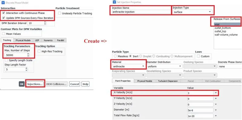
- Interaction:-
- Interaction with continuous phase => Enable
- This allows the both continuous phase & discrete phase to influence each other. Solves the discrete and continuous phase equations until the solutions in both phases stop changing.
- DPM sources are updated for every 10 iteration interval.
- Interaction with continuous phase => Enable
- Tracking parameters:-
- Maximum Number of steps = 50000
- This factor is used to abort trajectory calculations when the particle never exits the flow domain and reports the trajectory fate as "incomplete''. The limit on the number of integration time steps eliminates the possibility of a particle being caught in a recirculating region of the continuous phase flow field and being tracked infinitely. The maximum number of steps can be increased up to a limit of 10e9 as per application.
- Maximum Number of steps = 50000
- Injections => create
- Name = anthracite injection
- Type = Surface injection
- Relese from => Inlet
- Material => anthracite
- Point Properties:
-
Particle Diameter (m) X-velocity (m/s) Air inlet velocity (m/s) Case_1.1 1e-6 3 3 Case_1.2 2e-6 3 3 Case_1.3 3e-6 3 3 Case_1.4 4e-6 3 3 Case_1.5 5e-6 3 3 Case_2.1 5e-6 1 1 Case_2.2 5e-6 2 2 Case_2.3 5e-6 3 3 Case_2.4 5e-6 4 4 Case_2.5 5e-6 5 5
-
- Cell zone conditions:-
- material name = air
- Boundary conditions:-
-
Type Momentum Discrete phase Boundary Condition Type Inlet Velocity inlet equal to injection velocity Reflect Outlet Top Pressure Outlet Guage pressure = 0 (Pa) Escape Outlet Bottom Pressure Outlet Guage pressure = 0 (Pa) Trap Wall Motion Shear Condition Discrete phase Boundary Condition Type Wall Stationary Wall No-slip Reflect - Reflect:- The particle rebounds off the boundary in question with a change in its momentum as defined by the coefficient of restitution.
-
Trap:- The trajectory calculations are terminated and the fate of the particle is recorded as "trapped''.
-
Escape:- The particle is reported as having "escaped'' when it encounters the boundary in question. Trajectory calculations are terminated.
- Reflect:- The particle rebounds off the boundary in question with a change in its momentum as defined by the coefficient of restitution.
-
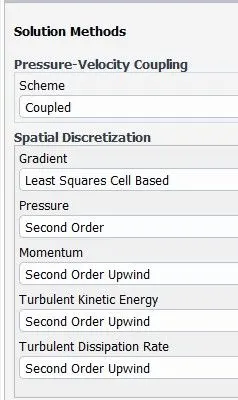
- Solution methods:-
- For more accurate results use a Second-order Upwind Spatial Discretisation scheme for Turbulent kinetic Energy and Turbulent Dissipation Rate.
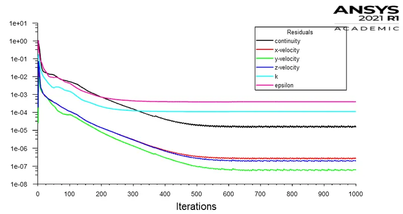
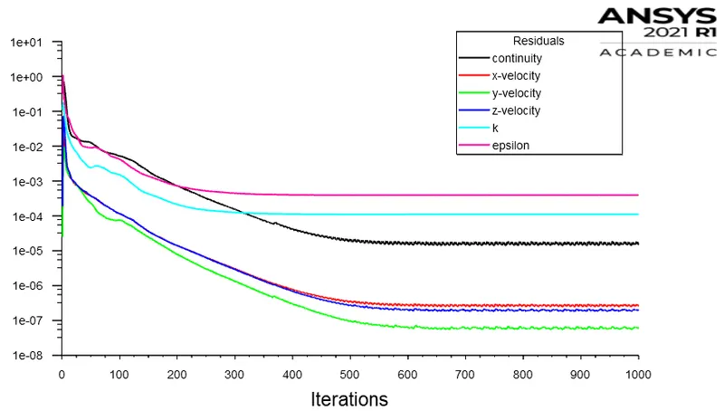
- Residual monitors:
- uncheck the convergence
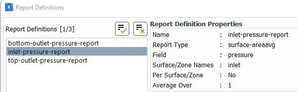
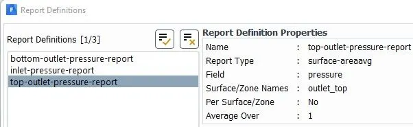
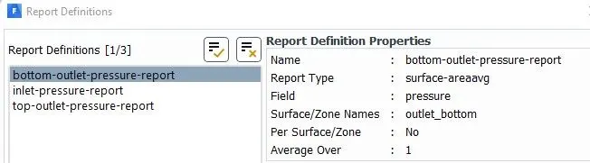
- Report Definitions:-
- Inlet Pressure monitor
-
- Outlet Top Pressure monitor
-
- Outlet Bottom Pressure monitor
- Inlet Pressure monitor
- Initialization methods:-
- Standard Initialization
- Compute from = Inlet.
- Standard Initialization
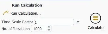
- Run Calculations:-
- Steady-State Simulation
- Steady-State Simulation
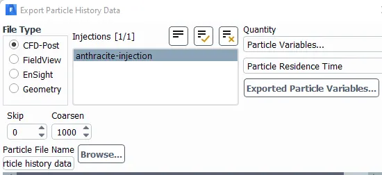
- Export
- Particle history data
- Particle history data



----------------------------------------------------------------------------------------------------------------------
4. Results:-
- Import FLUENT particle track file
- Creating Particle time, Velocity, and Pressure contours.
- Creating particle time animation.
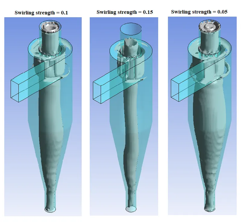
- Creating Vortex core region for swirling strength.
- Separation Efficiency:
- `text(Separation efficiency ) eta_s = text(Number particles traped)/text(Number particles tracked)`
- Pressure Drop:
- `text(Pressure Drop) = text(Inlet pressure - Outlet Pressure)`
----------------------------------------------------------------------------------------------------------------------
| Case_1.1 | ||
| Particle Diameter = 1e-6 m | X-velocity = 3 m/s | Air inlet velocity = 3 m/s |
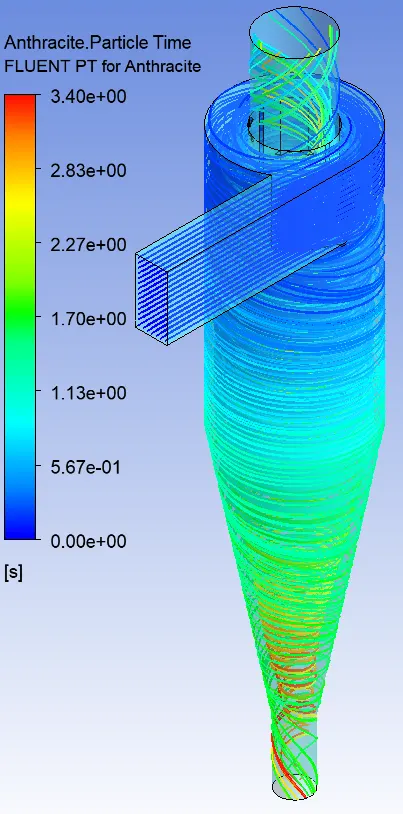
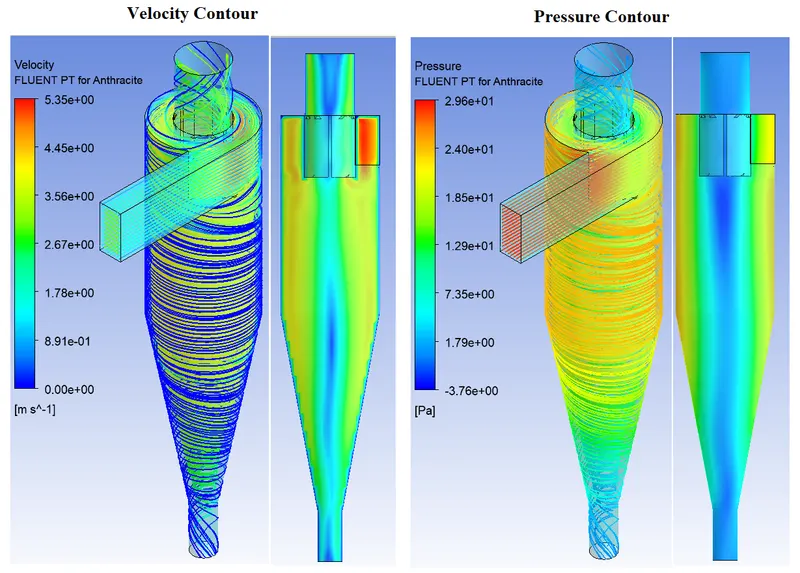

`eta_s = 25/98 = 0.2551 = 25.55%`
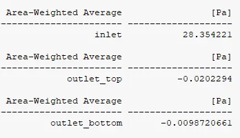
`text(P)_text(drop) = 28.354221-(-0.0202294) = 28.3744504 text( Pa)`
----------------------------------------------------------------------------------------------------------------------
| Case_1.2 | ||
| Particle Diameter = 2e-6 m | X-velocity = 3 m/s | Air inlet velocity = 3 m/s |
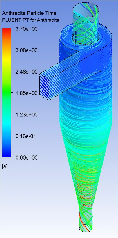
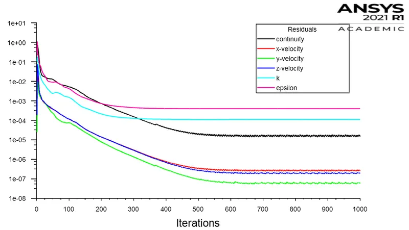
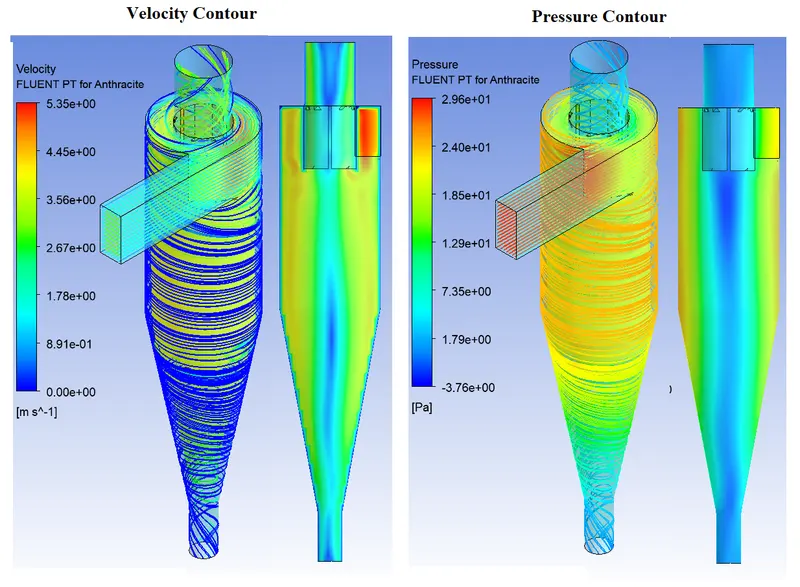

`eta_s = 60/98 = 0.6122 = 61.22%`
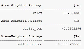
`text(P)_text(drop) = 28.354221-(-0.0202294) = 28.3744504 text( Pa)`
----------------------------------------------------------------------------------------------------------------------
| Case_1.3 | ||
| Particle Diameter = 3e-6 m | X-velocity = 3 m/s | Air inlet velocity = 3 m/s |
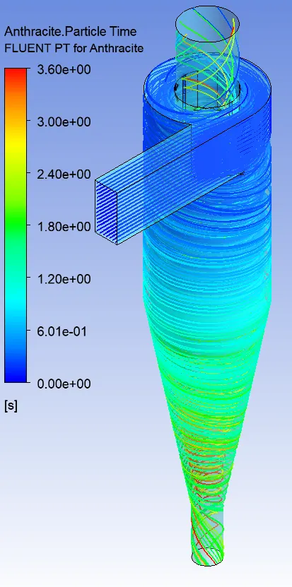
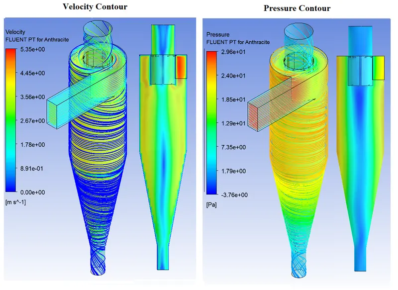

`eta_s = 75/98 = 0.7653 = 76.53%`
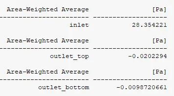
`text(P)_text(drop) = 28.354221-(-0.0202294) = 28.3744504 text( Pa)`
----------------------------------------------------------------------------------------------------------------------
| Case_1.4 | ||
| Particle Diameter = 4e-6 m | X-velocity = 3 m/s | Air inlet velocity = 3 m/s |
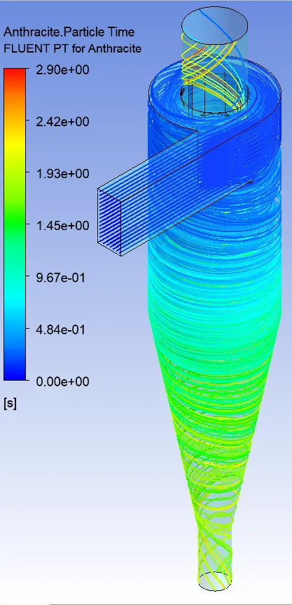
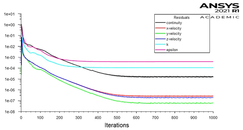
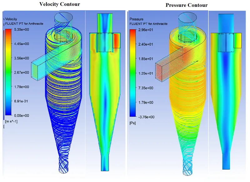

`eta_s = 85/98 = 0.8673 = 86.73%`
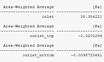
`text(P)_text(drop) = 28.354221-(-0.0202294) = 28.3744504 text( Pa)`
----------------------------------------------------------------------------------------------------------------------
| Case_1.5 | ||
| Particle Diameter = 5e-6 m | X-velocity = 3 m/s | Air inlet velocity = 3 m/s |
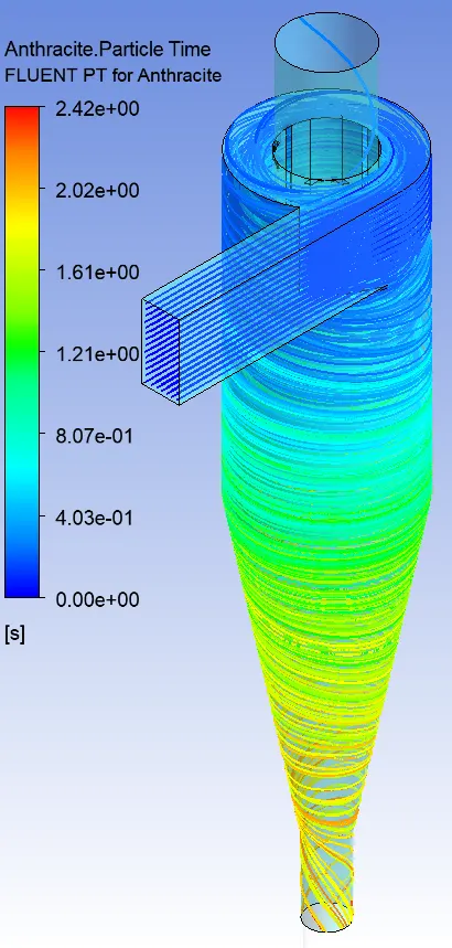
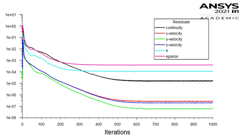
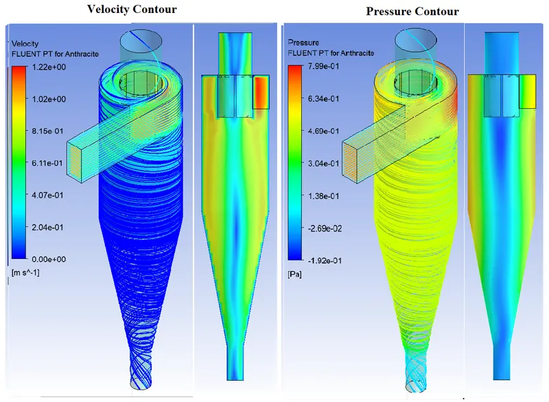

`eta_s = 95/98 = 0.9693 = 96.93%`
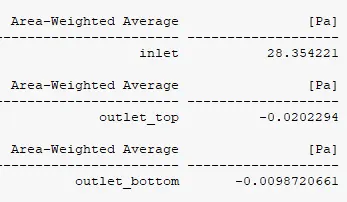
`text(P)_text(drop) = 28.354221-(-0.0202294) = 28.3744504 text( Pa)`
----------------------------------------------------------------------------------------------------------------------
----------------------------------------------------------------------------------------------------------------------
| Case_2.1 | ||
| Particle Diameter = 5e-6 m | X-velocity = 1 m/s | Air inlet velocity = 1 m/s |
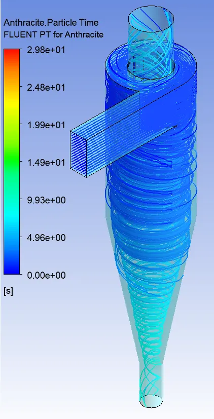
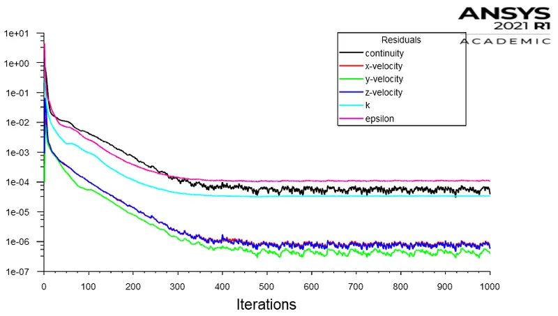
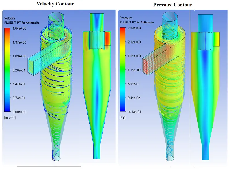

`eta_s = 8/98 = 0.0816 = 8.16%`
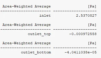
`text(P)_text(drop) = 2.5370827-(-0.000972558) = 2.538055258 text( Pa)`
----------------------------------------------------------------------------------------------------------------------
| Case_2.2 | ||
| Particle Diameter = 5e-6 m | X-velocity = 2 m/s | Air inlet velocity = 2 m/s |
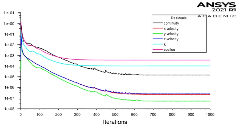
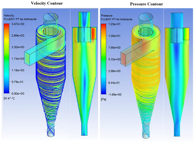

`eta_s = 47/98 = 0.4795 = 47.95%`
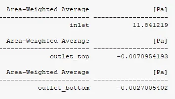
`text(P)_text(drop) = 11.841219-(-0.0070954193) = 11.8483144193 text( Pa)`
----------------------------------------------------------------------------------------------------------------------
| Case_2.3 | ||
| Particle Diameter = 5e-6 m | X-velocity = 3 m/s | Air inlet velocity = 3 m/s |
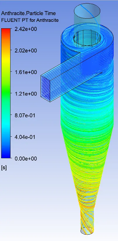
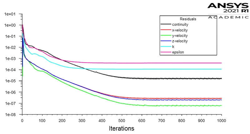
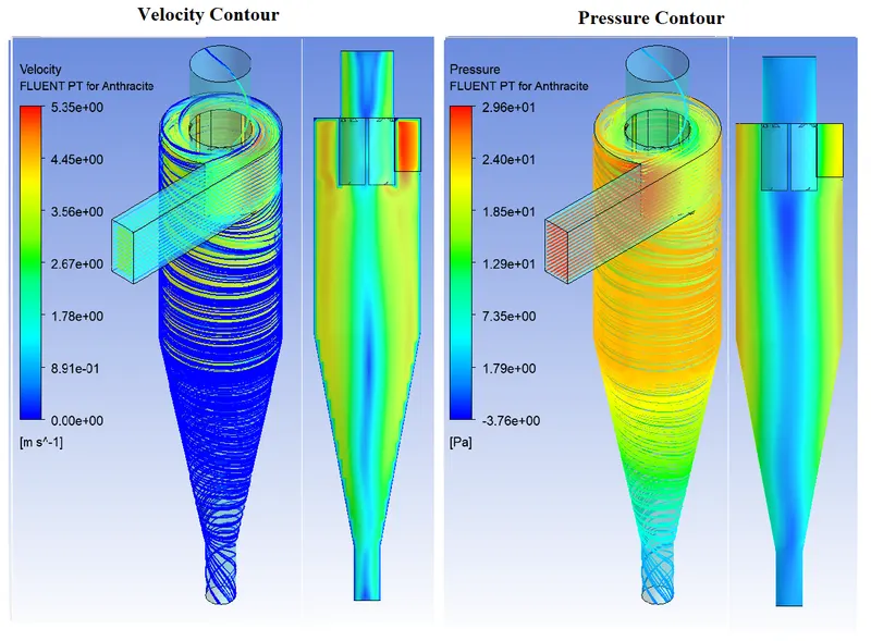

`eta_s = 95/98 = 0.9693 = 96.93%`
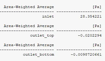
`text(P)_text(drop) = 28.354221-(-0.020229) = 28.37445 text( Pa)`
----------------------------------------------------------------------------------------------------------------------
| Case_2.4 | ||
| Particle Diameter = 5e-6 m | X-velocity = 4 m/s | Air inlet velocity = 4 m/s |
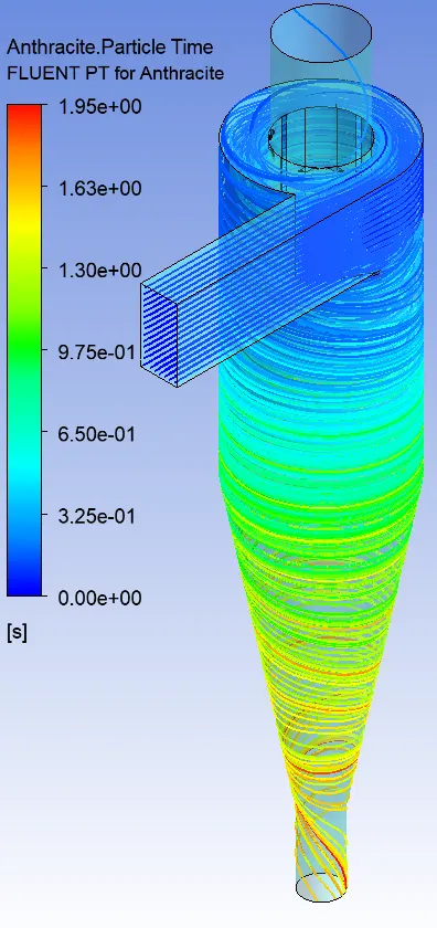
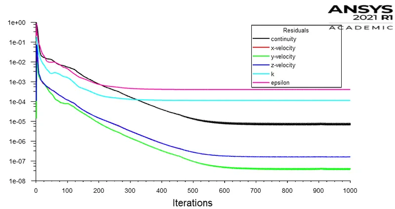
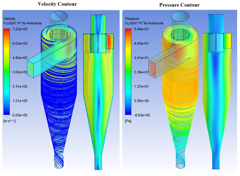

`eta_s = 95/98 = 0.9693 = 96.93%`
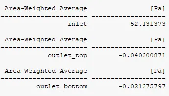
`text(P)_text(drop) = 52.131373-(-0.040300871) = 52.171673871 text( Pa)`
----------------------------------------------------------------------------------------------------------------------
Vortex Core region:
----------------------------------------------------------------------------------------------------------------------
Result table:| Particle Diameter (m) | X-velocity (m/s) | Air inlet velocity (m/s) | Particles Tracked | Particles Traped | Particles Escaped | Particles Incomplete |
Separation Efficiency = Traped/Tracked % |
Inlet Pressure [Pa] | Top Outlet Pressure [Pa] | Pressure Drop [Pa] | Bottom Outlet pressure [Pa] | |
| Case_1.1 | 1e-6 | 3 | 3 | 98 | 25 | 38 | 35 | 25.55 | 28.3454 | -0.0202 | 28.3744 | -0.0098 |
| Case_1.2 | 2e-6 | 3 | 3 | 98 | 60 | 33 | 5 | 61.22 | 28.3454 | -0.0202 | 28.3744 | -0.0098 |
| Case_1.3 | 3e-6 | 3 | 3 | 98 | 75 | 23 | 0 | 76.53 | 28.3454 | -0.0202 | 28.3744 | -0.0098 |
| Case_1.4 | 4e-6 | 3 | 3 | 98 | 85 | 13 | 0 | 86.73 | 28.3454 | -0.0202 | 28.3744 | -0.0098 |
| Case_1.5 | 5e-6 | 3 | 3 | 98 | 95 | 3 | 0 | 96.96 | 28.3454 | -0.0202 | 28.3744 | -0.0098 |
| Case_2.1 | 5e-6 | 1 | 1 | 98 | 8 | 26 | 64 | 8.16 | 2.5370 | -0.0009 | 02.5380 | -0.00004 |
| Case_2.2 | 5e-6 | 2 | 2 | 98 | 47 | 6 | 45 | 47.95 | 11.8412 | -0.0070 | 11.8483 | -0.0027 |
| Case_2.3 | 5e-6 | 3 | 3 | 98 | 95 | 3 | 0 | 96.93 | 28.3542 | -0.0202 | 28.3744 | -0.0098 |
| Case_2.4 | 5e-6 | 4 | 4 | 98 | 95 | 3 | 0 | 96.93 | 52.1313 | -0.0403 | 52.1716 | -0.0213 |
----------------------------------------------------------------------------------------------------------------------
Solution Animations:-
- Vortex Core strength:
----------------------------------------------------------------------------------------------------------------------
Conclusions:-
- The separation efficiency of the cyclone separator increases with an increase in Particle Size and Inlet Velocity.
- As the inlet velocity increases Pressure drops and separation efficiency increases.
- For Smaller velocity values and for tiny particle sizes most of the particles entered into recirculation mode.