Week 8- Moving zones approach in Fluent

AIM: To understand the concept of Model Moving Zones and perform simulate Rotary motion for the given model and plot the velocity profile of the fluid motion.

Introduction:

There are two approaches to model rotary motion:

• Moving Reference frame.
• Moving Mesh approach.

Moving Reference frame (MRF) :

The MRF technique involves transforming the governing equations from the global or absolute reference frame to a local or relative reference frame that moves with a specified angular or translational velocity.

This transformation simplifies the equations and allows for the modeling of rotating or moving components without explicitly simulating their motion.

• In this approach, the frame is moving, and the Mesh topology remains the same.
• It's a steady phenomenon, no change in volume occurs.
• This method is preferred if unsteadiness is not important.

Moving Mesh Method(MMM) :

The Moving Mesh Method is a numerical technique used in computational simulations, particularly in the field of computational fluid dynamics (CFD) and structural analysis. This method involves dynamically adjusting the computational mesh during the simulation to adapt to the evolving geometry or flow field. The primary goal is to capture and resolve the evolving features of the solution more efficiently than a fixed mesh would allow.

• In, this approach the Mesh is moving, and the topology changes with time.
• It's an Unsteady Phenomenon, and the control volumes changes with time.
• This method is preferred if unsteadiness is significant.

Simulate rotary motion for the given geometry:

Simulation setup:

First, load the given 2D geometry into the Fluent setup. Here the model is pre-meshed with a fine meshing setup.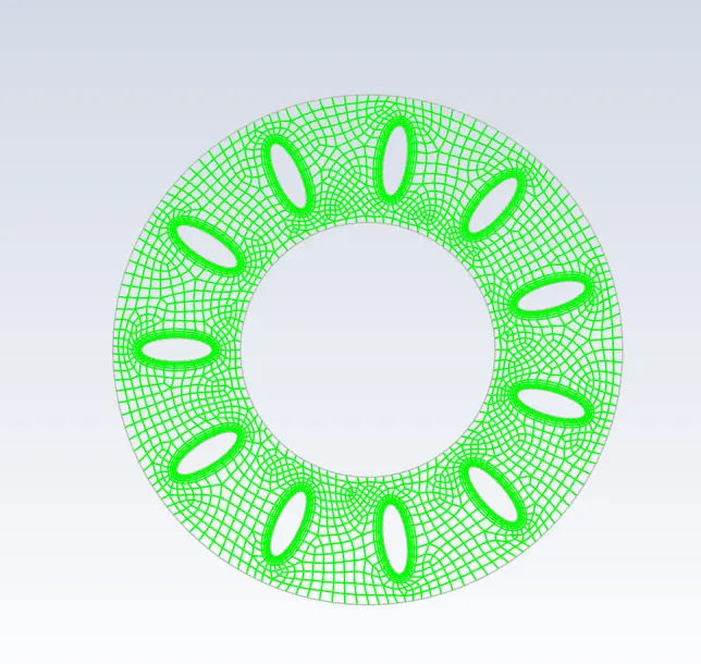

General:

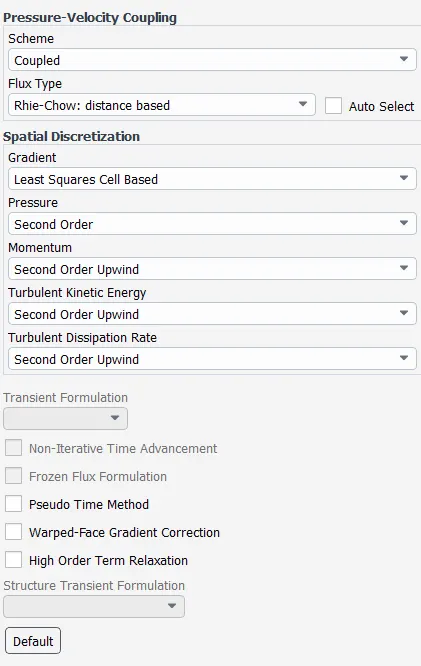
This stimulation is a steady-state simulation, and a pressure based solver is taken.

Turbulence models:

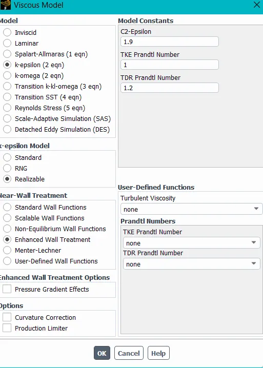
Cell zone conditions:

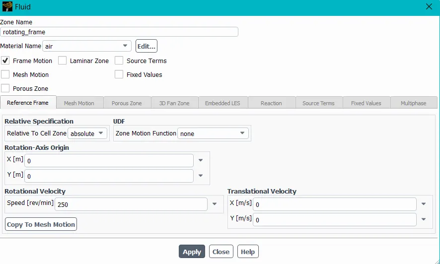
In this simulation, moving reference Frame method is taken and here, the rotating frame has a velocity of 250rpm.

Material:

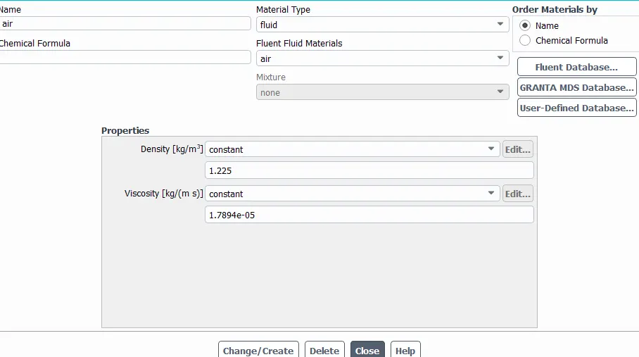
Here, the fluid material is taken as air having constant properties.

Boundary conditions:

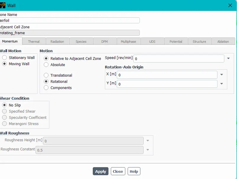
And the Boundary conditions of the air foils walls as moving walls of rotational motion type.

Solution Methods:

Results:

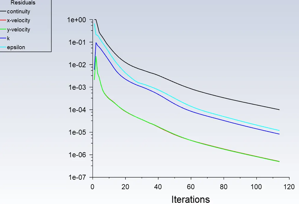
Residuals:

Pressure contour:

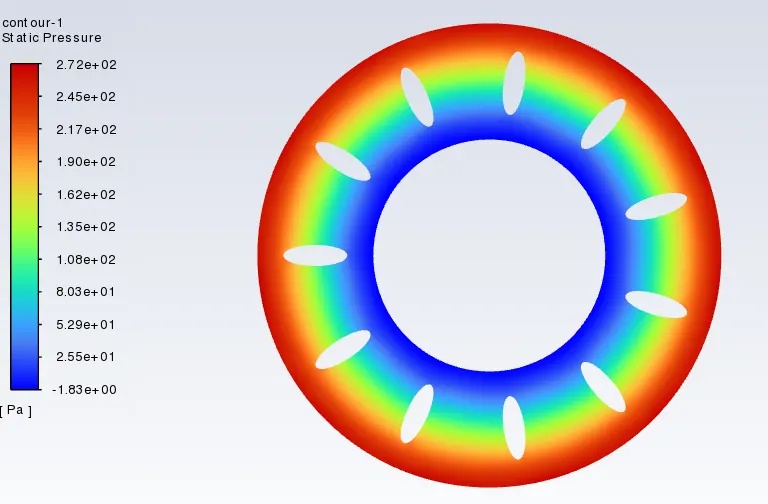
Here, the pressure contour results in high static pressure at the Outer circle of the model. And a negative static Pressure near the inner circle of the model.

Velocity contour:

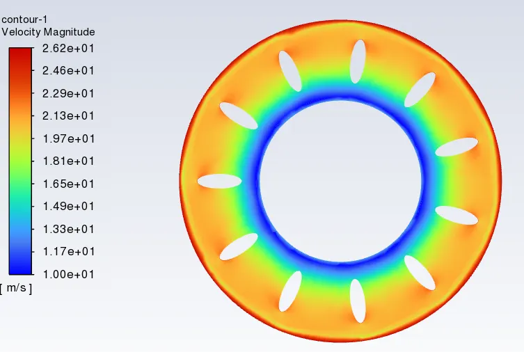
The high velocity noticed at the outer edges of the model that equal to 26.2m/sec, and at the inner edges of the circle the velocity is 10m/sec. And also at the edges of the every airfoil, the high velocity regions are occurred.

Velocity vector:

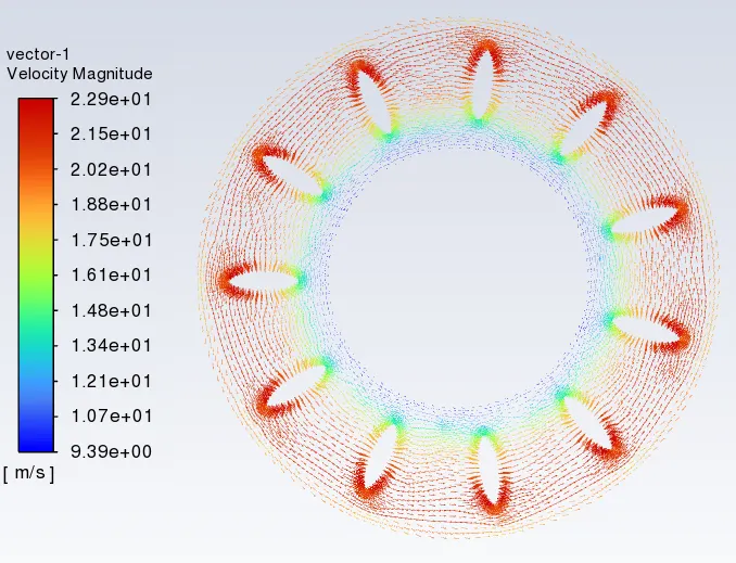
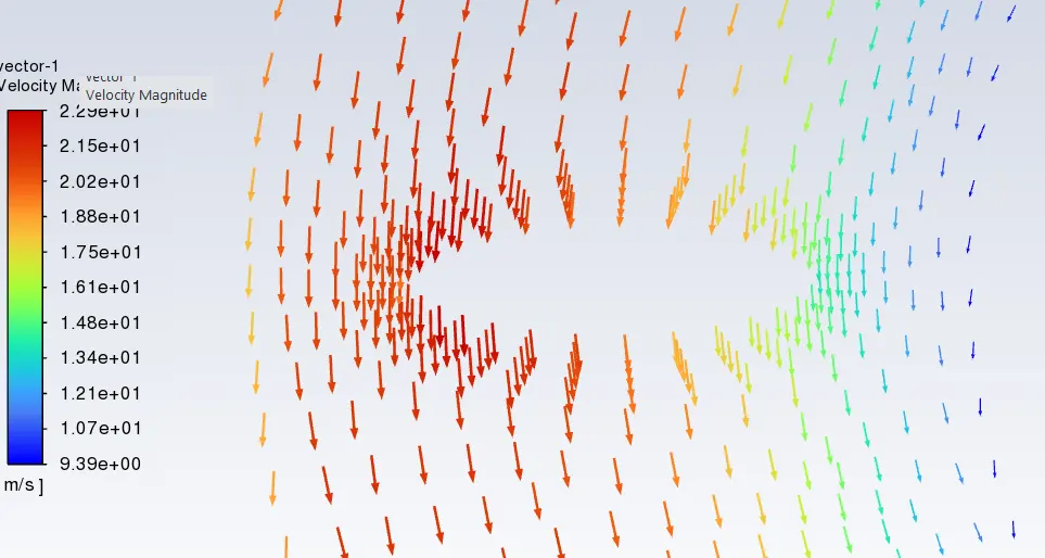
Here, the maximum velocity vector is occurred at the edges of the airfoil and collision of fluid occurs at the airfoil region.