Week 8- Moving zones approach in Fluent
What are the approaches by which you would model moving zones?
Two types of motoin involved in fluid flow are as follows
- Rotational Motion
- Rectilinear Motion
Rotational motion in CFD is modelled by the following approaches.
- Moving Reference Frame (MRF)
- Moving Mesh Method (MMM)
Navier stokes equation is solved separately in the stationary & moving frame zones. Data is transferred from one frame to another frame through the interface by using following methods to solve Momentum, Energy & Mass Equations.
- Area averaging method
- Mass averaging method
- mixed out approach (best of all other method, as no averaging is done)
A) Moving Reference Frame (MRF): It is steady state CFD modelling approach for simulating rotating equipments. A thin volumetric region of mesh cells is created around the rotating body during the meshing phase. This region is known as the MRF zone. During the simulation phase, the MRF zone is rotated about the axis of the body and the body is kept stationary. In order to preserve the direction of Coriolis Forces on the body.
- Single Reference Frame: The Entrie Computational domain is assumed to be single frame of approach.
- Multiple Reference Frame: In complex geometry it is not possible to use a single reference frame. In such cases break the problem into multiple cell zone with well defined interfaces between the cell zones.
B) Moving Mesh Method (MMM): It is used in simulation where sliding & deforming mesh is present. MMM are adaptive techniques for solving PDE's to improve the approximation of the solution.
- Sliding Mesh Method: Fluid interation between the stationary & Moving parts to employ the sliding mesh method to capture the transient behaviour of the fluid flow.
Which approach would you use to model unsteady phenomena?
Unsteady Phenomena is usually modelled using Moving Mesh Method
Simulate rotary motion for the geometry given
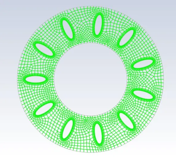
Mesh File:
- Open Ansys Fluent >> Import the mesh file.
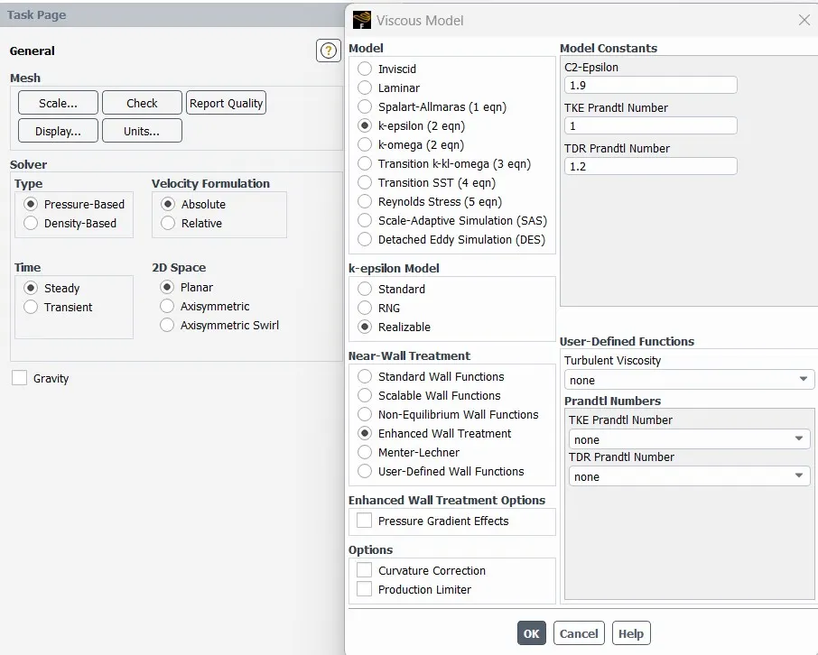
- In the general setting we are going for 2D Planar Steady state Pressure based simulation.
- Viscous model: K-epslion, Realizable, enhanced wall treatment. we could also go for K-omega turbulence modelling also.
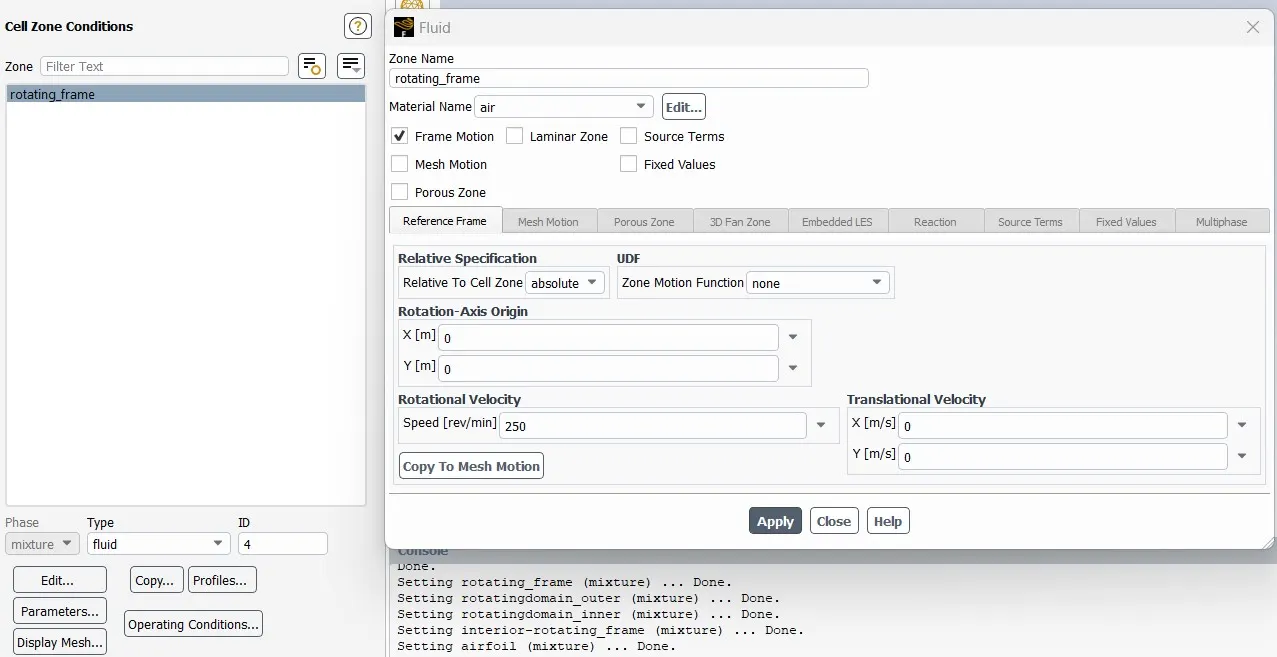
- Since we are study the Moving Reference frame method or Single refernce frame model (SRF) so, we initiate the rotating frame in rotational motion with 250rpm under cell zone condition.
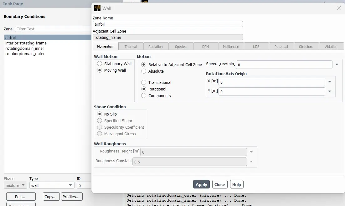
- Aerofoil is given moving wall rotational boundary condition, where the motion is induced to the aerfoil by the relative motion of the adjacent cell zone hence RPM is not mentioned.
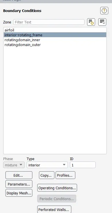
- Interior of the model is given interior boundary condition.
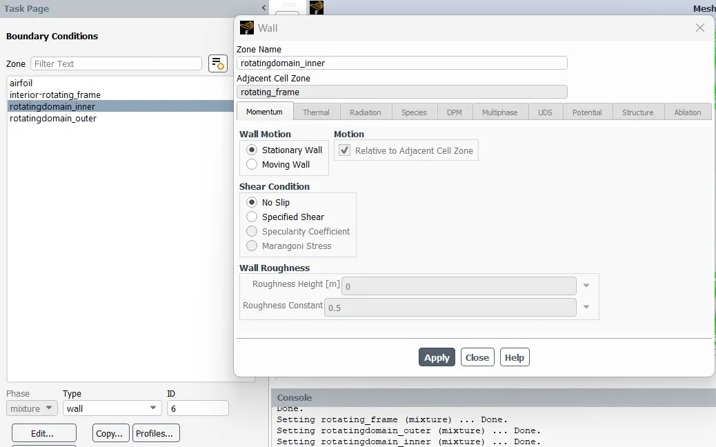
- Models inner boundary is given stationary wall boundary condition.
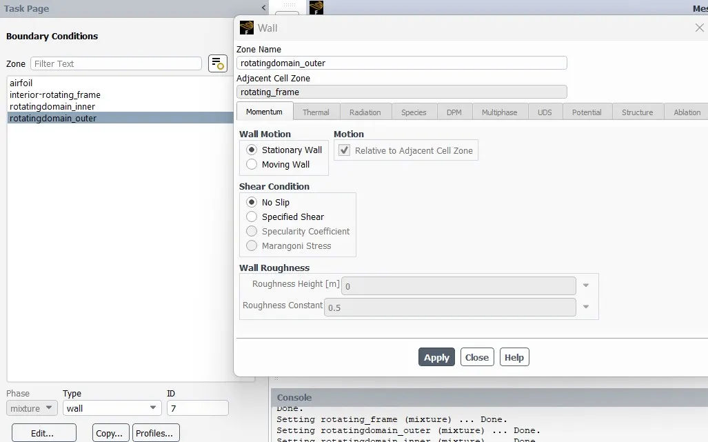
- Models outer boundary is given stationary wall boundary condition.
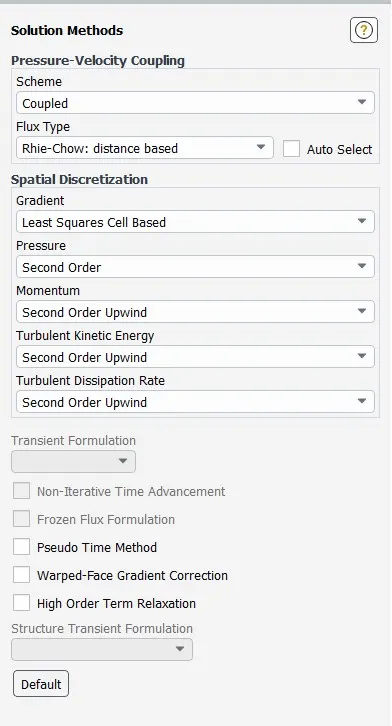
- Perssure Velocity coupling method and 2nd order upwind method is used.
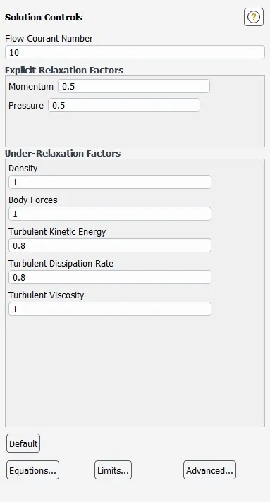
- Courant number is said to be 10.
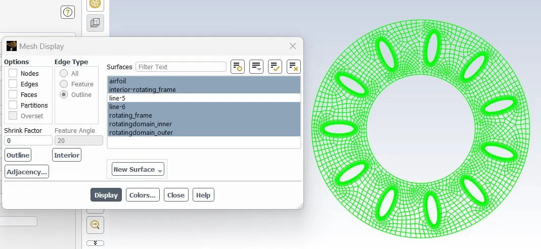
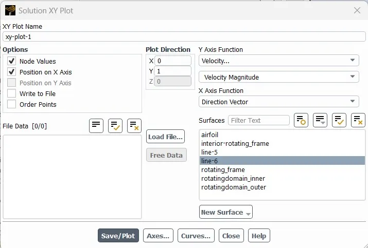
- Line is drawn on the model to plot the parameters along the line direction. So, vertically a line is plot on the model
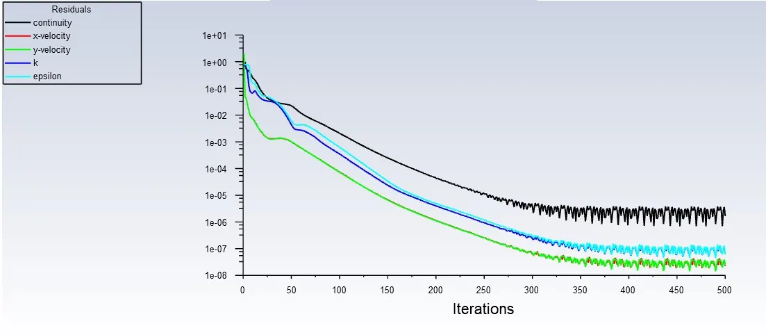
Result: The Simulation is run for 500 iterations
Residual:
XY Plot:
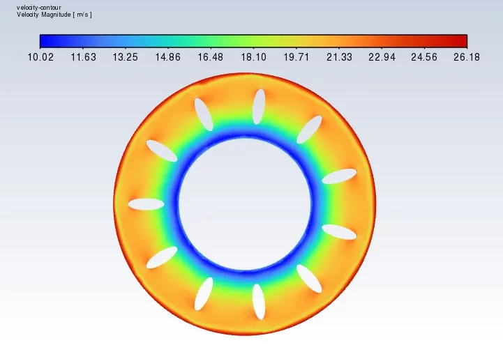
Velocity Contour:
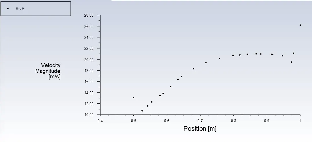
Velocity Plot along the Radial Direction:
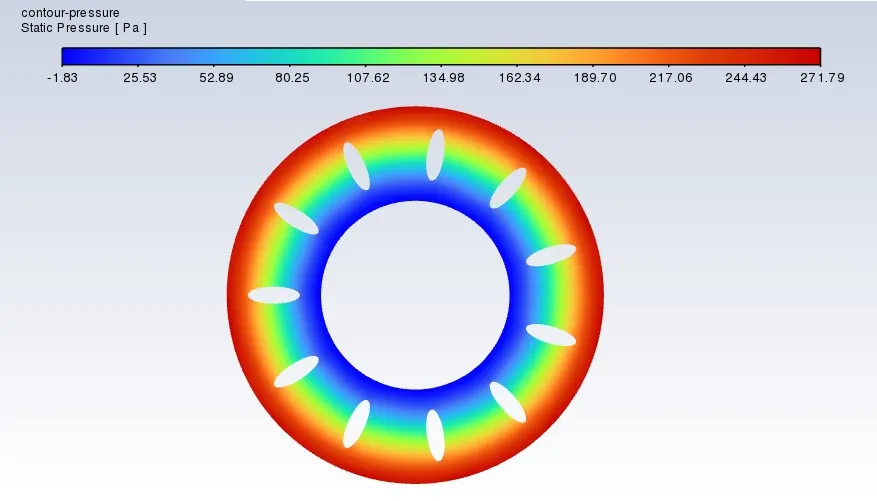
Static Pressure Contour:
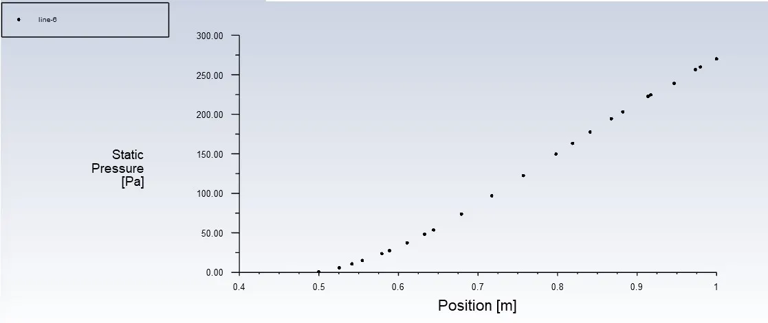
Static Pressure Plot along the Radial Direction:
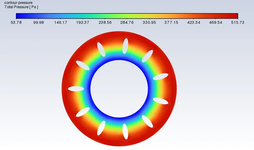
Total Pressure Contour:
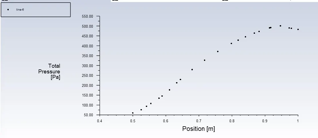
Total Pressure Plot along the Radial Direction:
Conclusion:
- From the Simulation we have found that the at the outer wall velocity of fluid is high.
- Static Pressure at the inner wall falls below atmospheric pressure.
| Sr. No. | Parameters | Minimum | Maximum |
| 1 | Velocity | 10.016 m/s | 26.177 m/s |
| 2 | Static Pressure | -1.833 Pa | 271.789 Pa |
| 3 | Total Pressure | 53.781 Pa | 515.731 Pa |