Week 8- Moving zones approach in Fluent

Aim- To study and simulate the rotary motion of geometry using the moving zones approach on Ansys fluent.

Objective-

• Explain motion zone approaches and their types.
• Which approach is suitable for the Model Unsteady state.
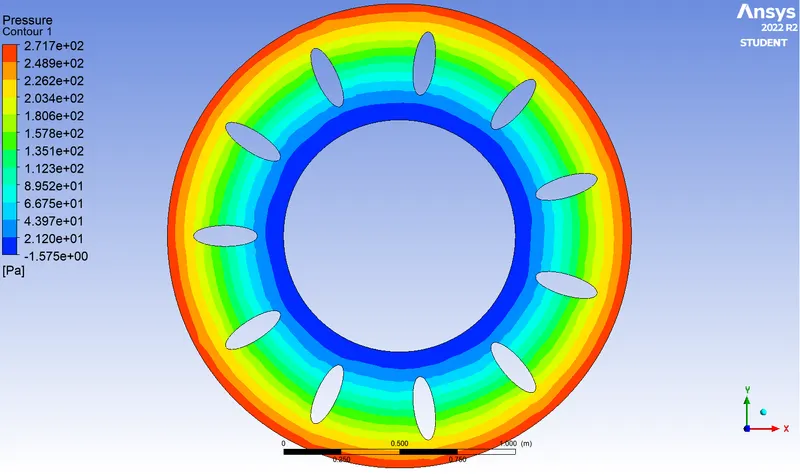
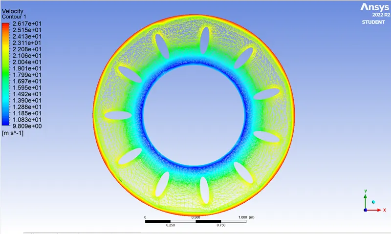
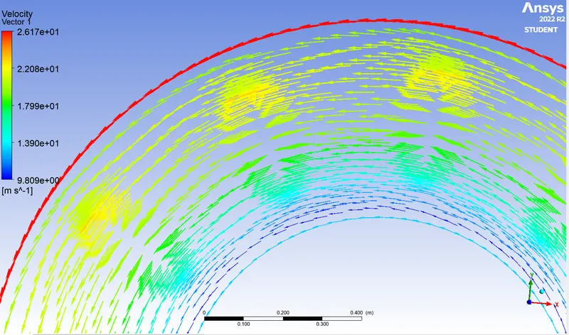
• Simulate the rotary motion of the geometry and plot a velocity profile of the fluid motion.

Theory-

Moving Cell Zones-

The solution of flows in moving reference frames requires the use of moving cell zones. This cell zone motion is interpreted as the motion of a reference frame to which the cell zone is attached.

Model moving zones approaches are-

1. Multiple Reference Frame Model(MRF)
2. Mixing Plane Model
3. Sliding mesh model

MRF formulation depends on two formulations-

• Relative Velocity Formulation
• Absolute Velocity Formulation

Relative Velocity Formulation

In FLUENT’s implementation of the multiple reference frame feature, the calculation domain is divided into subdomains, each of which may be rotating/translating with respect to the laboratory (inertial) frame. The governing equations in each subdomain are written with respect to that subdomain’s reference frame.

At the boundary between two subdomains, the diffusion and other terms in the governing equations in one subdomain require values for the velocities in the adjacent subdomain. FLUENT enforces the continuity of the absolute velocity,, to provide the correct neighbour values of velocity for the subdomain under consideration.

When the relative velocity formulation is used, velocities in each subdomain are computed relative to the motion of the subdomain. Velocities and velocity gradients are converted from a moving reference frame to the absolute inertial frame.

Absolute Velocity Formulation

When the absolute velocity formulation is used, the governing equations in each subdomain are written with respect to that subdomain’s reference frame, but the velocities are stored in the absolute frame. Therefore no special transformation is required at the interface between two subdomains.

Moving Reference Frame Model(MRF)

A Moving Reference Frame (MRF) is a relatively simple, robust, and efficient steady-state, Computational Fluid Dynamics (CFD) modelling technique to simulate rotating machinery.

A steady-state approach used in industrial computational fluid dynamics to model challenges with rotating components is the Moving Reference Frame (MRF) approach. It is thought to need less computer power while being efficient enough for most industrial situations.

This strategy’s underlying principles are straightforward but elegant. During the meshing phase, a small volumetric zone of mesh cells is produced around the spinning body, and the MRF zone encompasses this area.

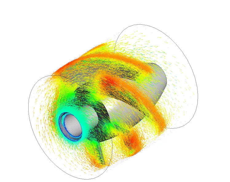
The MRF zone is rotated around the body’s axis while the body remains still during the simulation phase. In a reference frame that rotates or moves at the same speed as the rotating or moving geometry, governing equations are solved. On a physical level, it means that we see the flow field around the moving body while seated on it. The flow field becomes stable concerning the geometry as a result.

When a turbine is rotating and we are on the ground, the flow field surrounding the turbine seems transitory to us. If we sat on a turbine blade and rotated with it, instead of seeing it from a distance, the flow field around us or the turbine would appear stable.

For the model steady Phenomenon, we use,

The Moving Reference Frame Model(MRF) is used for Steady Phenomenon

• Frame is moving
• Mesh Topology Remains the Same
• No change in the control volume
• Steady Phenomenon
• If Unsteadiness is not important

For the model Unsteady Phenomenon, we use,

The moving Mesh Approach is used for Unsteady Phenomenon, and when we have a rotating wall that will change skewness of your element.

Used for Modelling Unsteady Phenomenon such as

• Vortex Induced Flows
• Interaction of Vortex with bodies
• Mesh is moving
• Toplogy Changes with Time
• Control Volume Changes with Time
• Unsteady Phenomenon
• If Unsteadiness is important

Setup-

• Import the mesh geometry on the Ansys fluent and setup the simulation constraints.
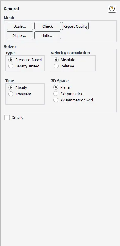
• General setup -

Steady-state Analysis

Pressure Based solver

2d State - planar

Velocity formulation - absolute

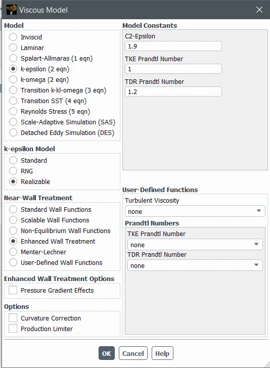
• Viscous model = K-epsilon model - Realiazable - Enhanced wall treatment

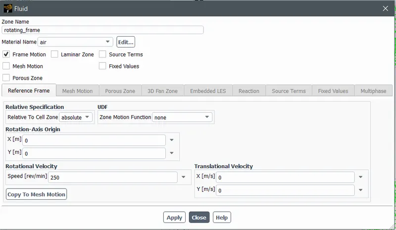
• Cell zone conditions = Rotating frame- Frame motion- Rotational velocity -250 rpm

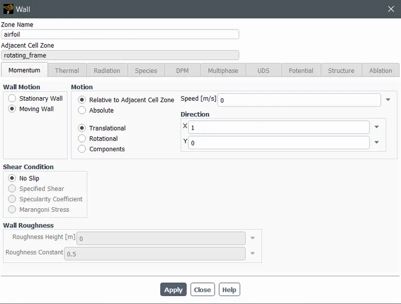
• Boundary conditions = Walls - moving wall

Relative to adjacent cell zones - Rotational

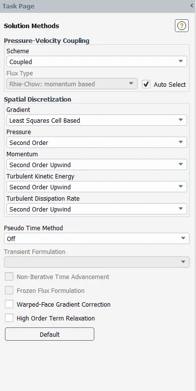
• Methods - Coupled Scheme

second-order upwind model

• Controls = Flow cournat number= 10
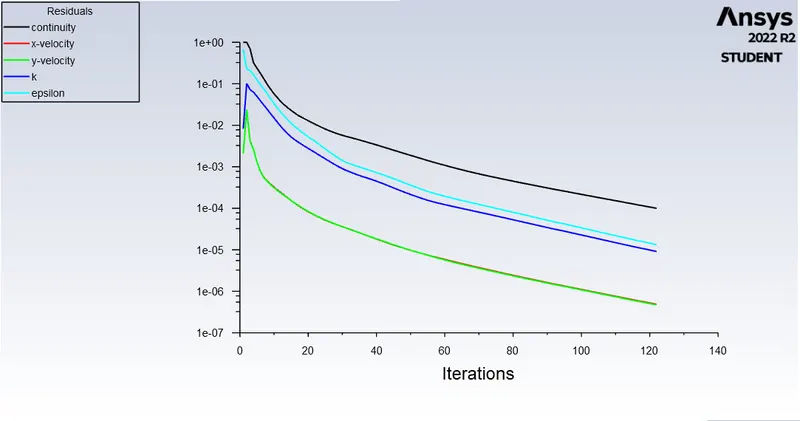
• we go with Hybrid Initialization and number of iteartions = 500

• The solution got converged at 120th iterations.

Conclusion-

• Understanding the Moving zones approaches.
• For simulating a moving Zones approach for a steady-state simulation MRF approach is considered.
• Understand which approach is suitable for steady and unsteady state simulation.