Week 8- Moving zones approach in Fluent

Week 8- Moving zones approach in Fluent

1. What are the approaches by which you would model moving zones?
2. Which approach would you use to model unsteady phenomena?
3. Simulate rotary motion for the geometry given
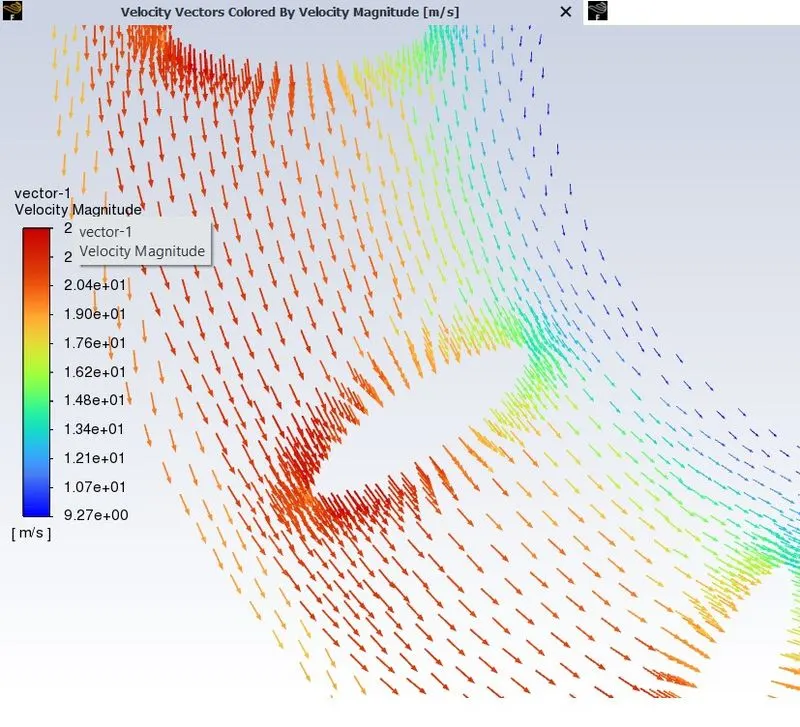
   1. Plot the velocity profile of the fluid motion

Answer

The two type of flow in in a fluid motion are rectilinear and rotary motion and there are two approaches to model these motions.

Moving reference frame approach and Moving mesh approach

Moving Reference Frame ( MRF)

A Moving Reference Frame (MRF) is a relatively simple, robust, and efficient steady-state, Computational fluid dynamics modeling technique to simulate rotating machinery. For example, the rotors on a quadcopter can be modeled with MRFs.

The principal reason for employing a moving reference frame is to render a problem which is unsteady in the stationary (inertial) frame steady with respect to the moving rame. For a steadily rotating frame (i.e., the rotational speed is constant), it is possible
to transform the equations of fluid motion to the rotating frame such that steady-state solutions are possible. By default fluent permits the activation of a moving refernce frame with a steady rotational speed. If the rotational speed is not constant, the transformed equations will contain additional terms which are not inclkuded in fluent formulation. unsteady simulations can be studied in moving refernce frame with constant rotational speed.

There are two types of moving refernce frame approach:

• Single moving refrence frame.
• Multiple moving refernce frame that uses a mixing plane approach.

contact region or the interface :

• this is the region existing in contact with the stationary plkane or the moving plane.
• Section or region of intersection of the two frames.
• Circuilar type of interface
• The Navier stokes equation is the stationary frame and the moving frame is solved separately.
• Data is tyransferred from one frame to another through interface

There are three methods of data transfer namely:

• Area averaging method

ϕ=(1A)∫e(ϕdA)ϕ=(1A)∫e(ϕdA)

• Mass avaeraging method:

ϕm=(1m)∫e(ρ⋅V⋅ϕ⋅dA)ϕm=(1m)∫e(ρ⋅V⋅ϕ⋅dA)

• Mixed approach

In this approach the partial differntiation equations are solved. the momentum equation, wenergy equation, the continiuty equation is solved simulataneouisly.

This approach gives the best result.

• Moving mesh approach is used to model unstaedy flows. Generally flows with vortex induced and for the flows for inetraction of vortex with the bodies, moving mesh approach is used. In moving mesh methods, physical PDEs and a mesh equation derived from equidistribution of an error metrics (so-called the monitor function) are simultaneously solved and meshes are dynamically concentrated on steep regions

Simulation

The Geometry. This is the geometry which we are going to deal today. This body remains fixed and the air flowing around it will be rotating at a speed of 250 rpm.

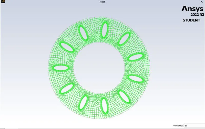
All these conditions are going to set as default since this is a basic problem

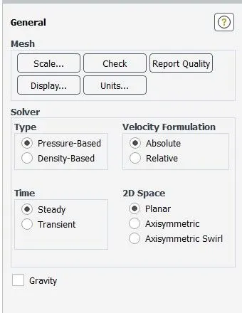
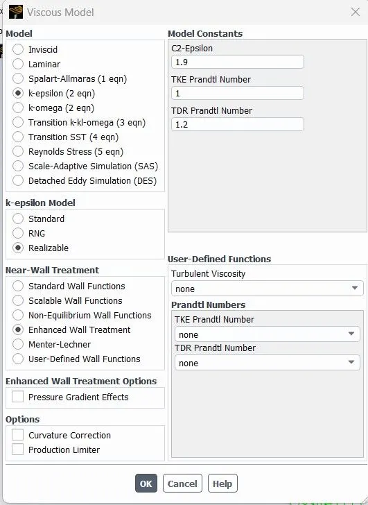
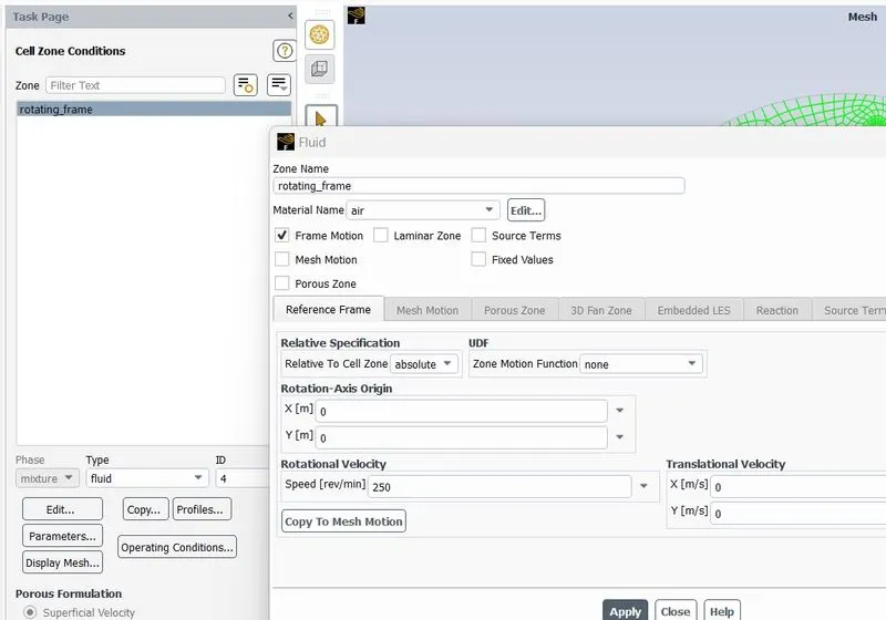
Frame Motion should be enabled in the cell zone conditions and the speed is set as 250 rpm.

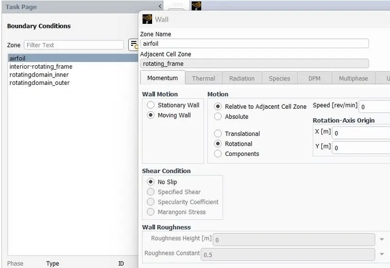
Moving wall condition is enabled in the Boundary condition for the airfoil section, and the motion is set to rotational.

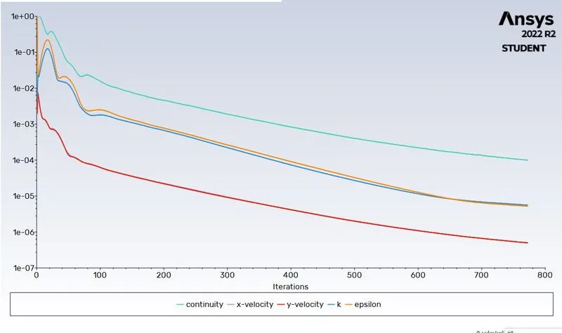
Residuals

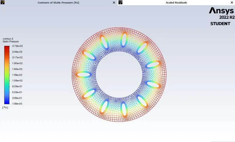
Static Pressure Contour of the simulation result

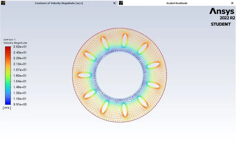
Velocity Contour

Picture Showing the directional vectors

Thank You