Week 8 - Simulation of a backward facing step in OpenFOAM
Aim
In this challenge, we are going to simulate an incompressible laminar-viscous flow through a backward-facing step geometry. We are solving it using an icoFoam solver for both laminar and incompressible flow.
Mesh
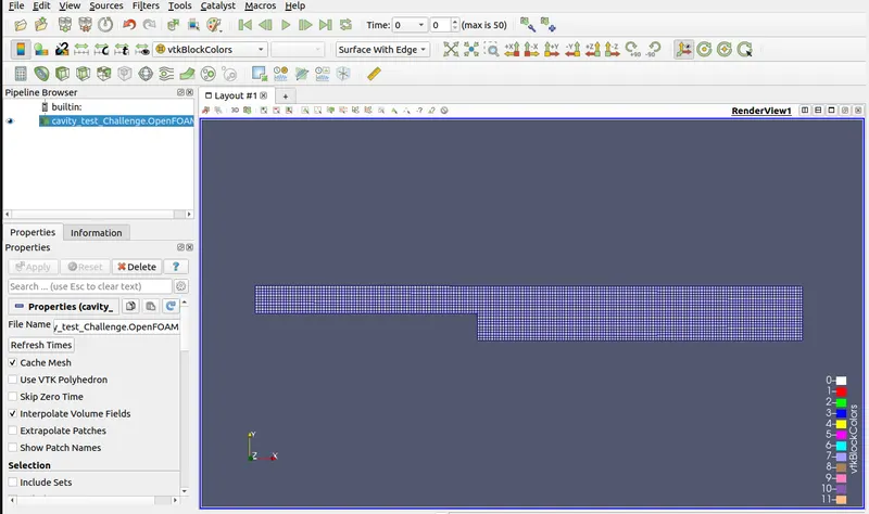
Number of cells along x-axis = 200
Number of Cells along y-axis = 20
Case 1, simulating the flow with a gradient factor of 1.
Boundary condition Specification
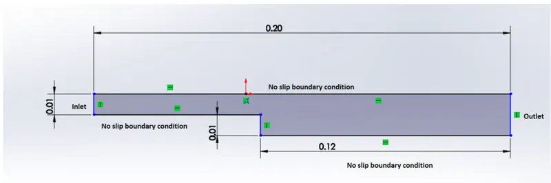
Geometry Creation
In order to solve a problem in OpenFOAM, we need to define certain parameters like initial conditions, geometry, and mesh.
Depending on the type of problem we are solving, we have to select the suitable case given in the tutorial folder. After selecting the solver, we have to copy the case file into a run folder, as OpenFOAM does not allow us to edit the tutorials.
Let us consider creating the geometry using 5 blocks as shown in the figure.

The Isometric view will be..
Each Node is defined with a node number.
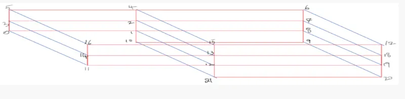
BLOCKMESHDICT.
/*--------------------------------*- C++ -*----------------------------------*\
========= |
\\ / F ield | OpenFOAM: The Open Source CFD Toolbox
\\ / O peration | Website: https://openfoam.org
\\ / A nd | Version: 9
\\/ M anipulation |
\*---------------------------------------------------------------------------*/
FoamFile
{
format ascii;
class dictionary;
object blockMeshDict;
}
// * * * * * * * * * * * * * * * * * * * * * * * * * * * * * * * * * * * * * //
convertToMeters 0.01;
vertices
(
(0 0 0)
(8 0 0)
(8 0.5 0)
(0 0.5 0)
(8 1 0)
(0 1 0)
(20 1 0)
(20 0.5 0)
(20 0 0)
(20 -1 0)
(8 -1 0)
(0 0 0.1)
(8 0 0.1)
(8 0.5 0.1)
(0 0.5 0.1)
(8 1 0.1)
(0 1 0.1)
(20 1 0.1)
(20 0.5 0.1)
(20 0 0.1)
(20 -1 0.1)
(8 -1 0.1)
);
blocks
(
hex (0 1 2 3 11 12 13 14) (80 5 1) simpleGrading (1 1 1)
hex (3 2 4 5 14 13 15 16) (80 5 1) simpleGrading (1 1 1)
hex (2 7 6 4 13 18 17 15) (120 5 1) simpleGrading (1 1 1)
hex (1 8 7 2 12 19 18 13) (120 5 1) simpleGrading (1 1 1)
hex (10 9 8 1 21 20 19 12) (120 10 1) simpleGrading (1 1 1)
);
edges
(
);
boundary
(
inlet
{
type patch;
faces
(
(0 11 14 3)
(3 14 16 5)
);
}
outlet
{
type patch;
faces
(
(9 8 19 20)
(8 7 18 19)
(7 6 17 18)
);
}
frontAndBack
{
type empty;
faces
(
(0 3 2 1)
(3 5 4 2)
(2 4 6 7)
(1 2 7 8)
(10 1 8 9)
(11 12 13 14)
(13 15 16 14)
(18 17 15 13)
(19 18 13 12)
(20 19 12 21)
);
}
NoslipWalls
{
type wall;
faces
(
(5 16 15 4)
(4 15 17 6)
(0 1 12 11)
(10 9 20 21)
(10 21 12 1)
);
}
);
mergePatchPairs
(
);
// ************************************************************************* //
MESH GENERATION
The is generated by running blockMesh command on this blockMeshDict file on the terminal. The status of the blockMesh is shown on the terminal window.
Boundary and Initial Condition
After creating the mesh, now the next step is to setup the Boundary and initial conditons. This can be done by editing the 'O' file, which is inside the case file.
Inside the 'o' file we can see two files 'P' (Pressure) and 'U' (velocity), which need to be edited according to the condition.
The initial condition for Pressure
/*--------------------------------*- C++ -*----------------------------------*\
========= |
\\ / F ield | OpenFOAM: The Open Source CFD Toolbox
\\ / O peration | Website: https://openfoam.org
\\ / A nd | Version: 9
\\/ M anipulation |
\*---------------------------------------------------------------------------*/
FoamFile
{
format ascii;
class volScalarField;
object p;
}
// * * * * * * * * * * * * * * * * * * * * * * * * * * * * * * * * * * * * * //
dimensions [0 2 -2 0 0 0 0];
internalField uniform 0;
boundaryField
{
inlet
{
type zeroGradient;
}
outlet
{
type fixedValue;
value uniform 0;
}
frontAndBack
{
type empty;
}
NoslipWalls
{
type zeroGradient;
}
}
// ************************************************************************* //
Initial Condition for Velocity
/*--------------------------------*- C++ -*----------------------------------*\
========= |
\\ / F ield | OpenFOAM: The Open Source CFD Toolbox
\\ / O peration | Website: https://openfoam.org
\\ / A nd | Version: 9
\\/ M anipulation |
\*---------------------------------------------------------------------------*/
FoamFile
{
format ascii;
class volVectorField;
object U;
}
// * * * * * * * * * * * * * * * * * * * * * * * * * * * * * * * * * * * * * //
dimensions [0 1 -1 0 0 0 0];
internalField uniform (0 0 0);
boundaryField
{
inlet
{
type fixedValue;
value uniform (1 0 0);
}
outlet
{
type zeroGradient;
}
frontAndBack
{
type empty;
}
NoslipWalls
{
type noSlip;
}
}
// ************************************************************************* //
Control Dict. File
Here we set the start time, end time and dt for the problem , here the start time is 0 and end time is 0.5, and we choose dt as .0005
/*--------------------------------*- C++ -*----------------------------------*\
========= |
\\ / F ield | OpenFOAM: The Open Source CFD Toolbox
\\ / O peration | Website: https://openfoam.org
\\ / A nd | Version: 9
\\/ M anipulation |
\*---------------------------------------------------------------------------*/
FoamFile
{
format ascii;
class dictionary;
location "system";
object controlDict;
}
// * * * * * * * * * * * * * * * * * * * * * * * * * * * * * * * * * * * * * //
application icoFoam;
startFrom startTime;
startTime 0;
stopAt endTime;
endTime 0.5;
deltaT 0.0005;
writeControl timeStep;
writeInterval 20;
purgeWrite 0;
writeFormat ascii;
writePrecision 6;
writeCompression off;
timeFormat general;
timePrecision 6;
runTimeModifiable true;
// ************************************************************************* //
Now, we have to view our results in a GUI based software called ParaView, by typing in the command paraFoam.
Before that, to compute the values we entered, we need to type in the solver we are using in the command window. The solver we are using is icoFoam.
After commanding the solver we need to type in paraFoam in the command window to open up the ParaView GUI software and to view the results.
The results obtained in the paraView will be like this.
Processing
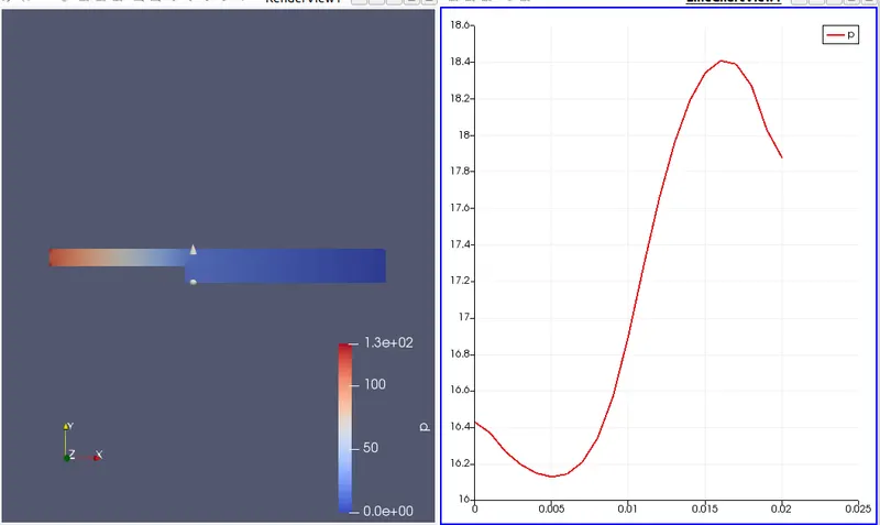
Results of the Pressure at 0.085m from the inlet, with a grading Factor of 1
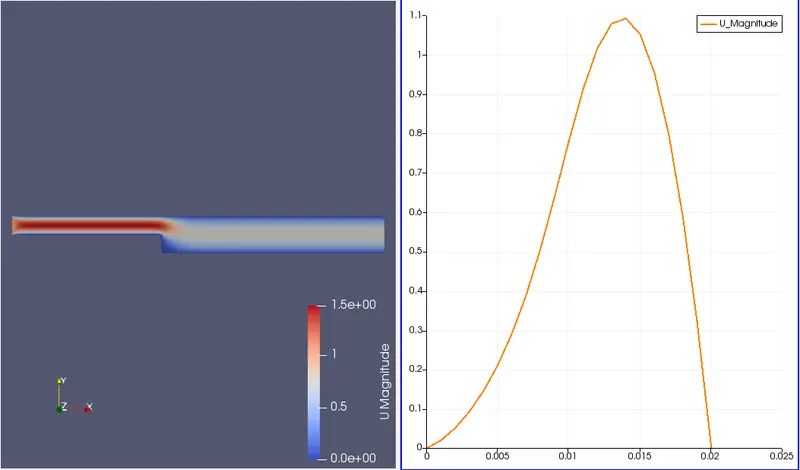
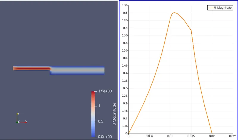
Results of the Velocity at 0.085m from the inlet, with a grading factor of 1.
CASE 2, Simulating the flow with a gradient factor of 0.2
Here, we are only just editing the blocMeshdict file only. Rest all are the same as case 1.
Here we are using a gradient factor of 0.2, that is changing the mesh refinement.
Gradient factor (f) = size of last cell (L) / size of First cell (F)
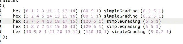
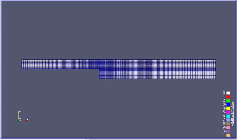
After editing the blockmeshdict file, in the command window, type in blockMesh , then checkMesh, then run the solver which is icoFoam. Now view the results in paraFoam.
The result obtained with a gradient factor of 0.02
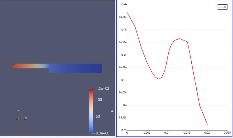
the results obtained for the pressure with a gradient factor of 0.2
The results obtained for the velocity is, with a gradient factor of 0.2
Conclusion
Here we can see that the plot with a gradient factor of 1 is smoother than the plot with a gradient factor of 0.2.
The grading factor gives us the freedom of generating refine mesh along particular direction which helps in most case to concentrate at a particular place. If the mesh is finer we will get information at that point will be almost with less simulation time.