Week 7 - Simulation of a 1D Super-sonic nozzle flow simulation using Macormack Method
Aim
To perform a program to solve the quasi 1D Subsonic- supersonic nozzle flow equations with the governing equations, in both conservative and non-conservative form.
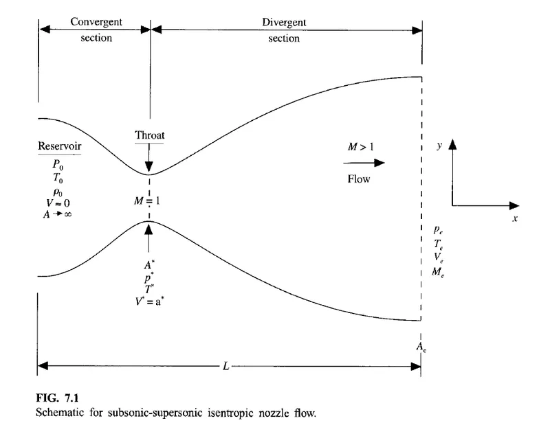
The entire material for this problem is taken from a book called 'Computational Fluid Dynamics - The basics with application' written by John D Anderson. This specific problem is in the 7th chapter of this book, section 7.3.
Here, we consider a situation of isentropic flow through a Convergent - Divergent nozzle. The fluid at the inlet of the nozzle is coming from a reservoir with a big(infinity) cross sectional area therefore the velocity at the inlet is very small(almost zero).
The flow expands isentropically to supersonic speed at the exit of the nozzle. In short , the fluid is subsonic in the convergent section , sonic at the throat area ( low cross section) and supersonic at the exit. Here, we are assuming that the flow is varying only along the x direction and not in any other direction, this type of flow is called quassi 1-D flow.
GOVERNING EQUATION IN THE NON-CONSERVATION FORM
The Governing equation can be expressed in two ways, the Conservative form and non- conservative form.
The non- conservative form of this problem is expressed as
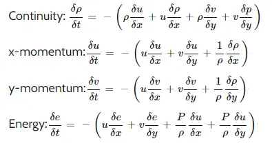
The 1-D Flow field variables are expressed as:-
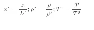
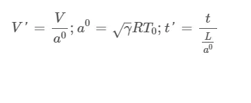
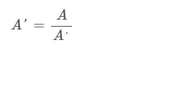
Where,
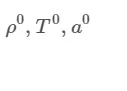 are the density, temperature and speed of sound at the reservoir.
A* is the throat area and L is the nozzle length.
Discretization
Here , the MacCormack technique is used for the discretization of the governing equation. The MacCormack method is an explicit finite difference method that is of second-order accurate in both space and time. For employing a time marching solution, which is of second order accurate, its is necessary to calculate the second order derivatives. Thus we uses a predictor - corrector method, that can produce second order accurate results without computing the second order derivatives. Thus it making much more simpler.
The predictor step computes the first order time derivative using the forward difference for spatial derivatives by substituting previous state values of the flow variables. It the updates the flow filed variables. These updated values are then used to compute corrector step time derivatives using the backward difference approach. Finally, the corrected solutions for the flow variables are obtained by using the average value of time derivatives computed in the predictor and corrector steps. These steps are repeated until a steady state is reached or until predefined time steps.
Now, we discretize the non-conservation equation form using MacCormack's Approach.
a) The predictor step
In the continuity equation , discretizing the spatial derivatives on the right hand side using the forward difference scheme.
Predicted value of density (rho)t+Deltat from the first two terms of Taylor series is as follows.

similarly
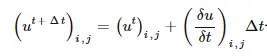
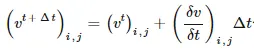

in the above equations, the numbers for the time derivative on the RHS are obtained from the equation.
b) Corrector step
In the corrector step, we use the computed predicted value of the time derivative at the time 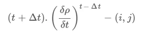
by substituting the values of rho,u,v into the RHS of the continuity equation.
Discretizing spatial derivatives by using a backward difference scheme.

The average value of the time derivative of density is obtained from the arithmetic mean of 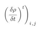 obtained in the equation.
This allows us to obtain the final corrected value of density at the time(t+deltat).
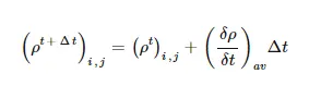
Similarly, we can calculate momentum and energy.
Nozzle shape and initial condition
The nozzle has a convergent-divergent shape with a length of 3 (non-dimensional).The nozzle area is minimum at the throat and it expands as we move towards the both end of the nozzle.
The defined area as a function of x,
A = 1+2.22(x-1.5)^2, 0<=x<=3
The initial condition must be chosen as close to the steady-state as possible. Otherwise, it can cause the solution can go unstable.
we know that the density and temperature increases and the velocity decreases as the flow expands inside the nozzle.
Therefore we chose the initial conditions that quantitatively describe the progressive increase and decrease.
At t=0
rho = 1-0.3146x
T = 1-0.2314x
V = (0.1 +1.09x)T^0.5
Boundary conditions
Inlet
At the subsonic inlet, we keep the rho and T fixed and allow V to float, i.e, it must be calculated as a function of timewise solution by linear extrapolation of inner nodes.
V(1) = 2*V(2)-V(3)
Outlet
at the supersonic outlet all the three flow field variables are allowed to float.
rho(n) = 2*rho(n-1) - rho(n-1)
V(n) = 2*V(n-1) - V(n-2)
T(n) = 2*T(n-1) - T(n-2)
With this information, a Matlab code can be performed, to simulate how the flow field variables vary across the nozzle with time.
GOVERNING EQUATION IN THE CONSERVATION FORM
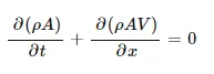
For the quassi 1-D subsonic-supersonic isentropic flow nozzle, the conservation form of energy equation can be expressed as.
continuity equation
Momentum equation
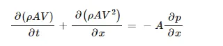
Energy equation

Expressing the above conservation form of equation using non-dimensional variables, we get..
Continuity equation
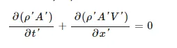
Momentum equation

Energy equation

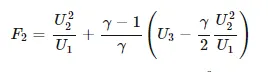
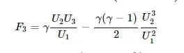
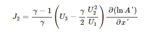
Let U be the solution vector, F be the flux vector, and J be the source term, such that.
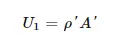
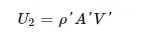
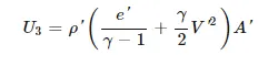
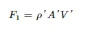
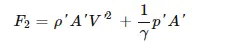

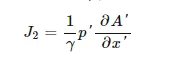
substituting these terms in the conservation form of equation, we get.
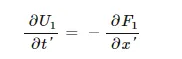
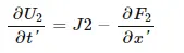
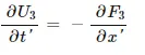
While writing the code we will solve for the solution vectors and then consecutively calculate the primitive variables using the following relations.
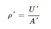
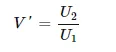
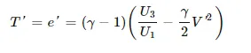
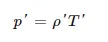
Now, we are solving for the solution vectors, the RHS consisting of flux terms and source terms must also be expressed in terms of U1,U2 and U3 to obtain the pure form of flux terms. Otherwise the solution may blow up after just few time steps.
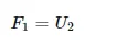
Discretization
Discretization of the governing equations in the conservation form will be done using MacCormack Method.
predictor step
The flux terms and source terms are calculate at nodes i and i+1 using previous state values of U1,U2 and U3 and forward difference is applied to compute the value of time derivatives.
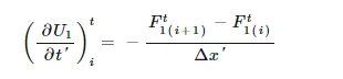

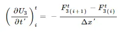
These time derivative values are used to calculate the predictor values of U1,U2 and U3.
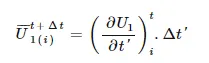
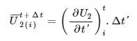
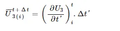
Corrector Step
A new set of flux and source term values are calculated using the predicted values of U1,U2 and U3 and backward difference is applied to compute the time derivative values for the corrector step.
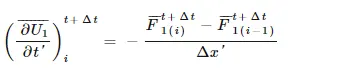

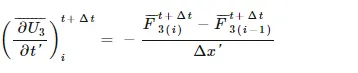
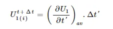
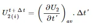
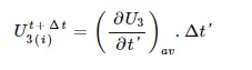
The average value of the predictor and corrector step derivative is calculated.



The corrected values of U1,U2 and U3 are computed using the average of derivative values.
Nozzle shape and Initial conditions
The nozzle shape and area is same as the previous one.
A = 1+2.22(x- 1.5)^2
Since the conservation from governing equations are more sensitive to the initial conditions, it is necessary to make them more realistic.
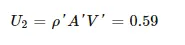
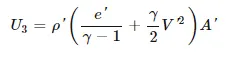
The variation of V for the initial condition can be synthesized by assuming a constant mass flow (U2) for initial conditions only, U2 = 0.59 is chosen for the initial condition
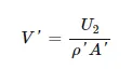
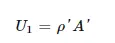
But the dependent variables being solved by the governing equations are U1,U2 and U3. We need initial conditions for them. The same initial conditions can be applied to U1,U2 and U3 using the relations.
Boundary Conditions
Inlet
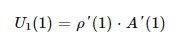
at the subsonic inlet, rho' and T' are fixed and V' is allowed to float.
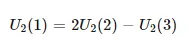
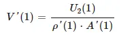
In terms of dependent variables, U1 will be fixed, U2 will float and U3 is a function of V' , It will also float.

Outlet
At the supersonic outlet, all the dependent variables are allowed to float.



with all the above information, we can write a Matlab program to solve quassi 1 D nozzle flow problem using both non- conservation and conservation forms.
Meshing
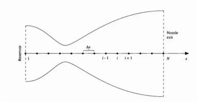
The first point 1 is assumed as the reservoir section, distributed along the x-axis with Delta x grid spacing. Point (I) is simply an arbitrary grid point with points(i-1) and (i+1) as the adjacent points.
For this problem, we are considering the number of grid points to be 31.
PPROGRAM
Main code
%main program for Quasi 1-D subsonic-supersonic nozzle flow.
clear all
close all
clc
%grid points
nx = 31;
L = 3; %length of the domain
%meshing
x= linspace(0,L,nx);
%grid spacing
dx = x(2)-x(1);
%nozzle area
A = 1+2.2*(x-1.5).^2;
gamma = 1.4;
nt = 1400;
C = 0.5; %courant number
% function for non conservative form
tic
[rho1,T1,V1,P1,M1,m1,rho_throat1,V_throat1,T_throat1,P_throat1,M_throat1,residual1]=Quasi_1D_nozzle_flow_non_conservative_func(x,dx,A,C,nt,gamma);
Time_taken_by_non_conservative_form = toc
%function for conservative form
tic
[rho2,T2,V2,P2,M2,m2,rho_throat2,V_throat2,T_throat2,P_throat2,M_throat2,residual2]=Quasi_1D_nozzle_flow_conservative_func(x,dx,A,C,nt,gamma);
Time_taken_by_conservative_form = toc
%plots for different variables
%plots for different flow parameters (non conservative form)
figure(1)
subplot(4,1,1)
plot(x,M1,'linewidth',2)
grid on
grid minor;
ax = gca;
ax.FontSize = 14;
ylim([0,4.5])
yticks(0:1.5:4.5)
ylabel('Mach Number','Fontsize',12,'Fontweight','bold')
title('non-conservative form of lowering equations','Fontweight','bold','color','g');
subplot(4,1,2)
plot(x,P1,'linewidth',2)
grid on
grid minor
ax = gca;
ax.FontSize = 14;
yticks(0:0.2:1)
ylabel('pressure ration','Fontsize',12,'Fontweight','bold')
subplot(4,1,3)
plot(x,rho1,'linewidth',2)
grid on
grid minor
ax = gca;
ax.FontSize=14;
yticks(0:0.2:1)
ylabel('Density ratio','Fontsize',12,'Fontweight','bold')
subplot(4,1,4)
plot(x,T1,'linewidth',2)
grid on
grid minor;
ax=gca;
ax.FontSize=14;
ylim([0,1]);
yticks(0:0.2:1)
ylabel('Temperature ratio','Fontsize',12,'Fontweight','bold')
xlabel('x/L','Fontsize',12,'Fontweight','bold')
%plots for different flow parameters(conservative form)
figure(2)
subplot(4,1,1)
plot(x,M2,'linewidth',2)
grid on
grid minor
ax=gca;
ax.FontSize=14;
ylim([0,4.5])
yticks(0:1.5:4.5)
ylabel('Mach nummber','Fontsize',12,'Fontweight','bold')
title('conservative form of lowering equations','Fontweight','bold','color','g')
subplot(4,1,2)
plot(x,P2,'linewidth',2)
grid on
grid minor
ax=gca;
ax.FontSize=14;
yticks(0:0.2:1)
ylabel('Pressure ratio','FontSize',12,'FontWeight','bold')
subplot(4,1,3)
plot(x,rho2,'linewidth',2)
grid on
grid minor;
ax=gca;
ax.FontSize = 14;
yticks(0:0.2:1);
ylabel('Density ratio','Fontsize',12,'Fontweight','bold')
subplot(4,1,4)
plot(x,T2,'linewidth',2)
grid on
grid minor;
ax=gca;
ax.FontSize=14;
ylim([0,1]);
yticks(0:0.2:1);
ylabel('Temperature ratio','Fontsize',12,'Fontweight','bold')
xlabel('x/L','Fontsize',12,'Fontweight','bold')
%plots for different flow parameters at throat section(non-conservative vs
%conservative form)
figure(3)
subplot(4,1,1)
plot(1:nt,M_throat1,'Linewidth',2)
hold on
plot(1:nt,M_throat2,'linewidth',2)
grid on
grid minor
ax=gca;
ax.FontSize=12;
yticks(0:0.2:1)
ylabel('Mach number','Fontsize',15,'Fontweight','bold')
l_g_d = legend('Non-conservative','conservative');
l_g_d.FontSize = 15;
title('Throat section of nozzle','FontSize',25,'Fontweight','bold','color','g')
subplot(4,1,2)
plot(1:nt,P_throat1,'Linewidth',2)
hold on
plot(1:nt,P_throat2,'Linewidth',2)
grid on
grid minor
ax=gca;
ax.FontSize = 12;
yticks(0:0.2:1)
ylabel('P/P_0','FontSize',15,'Fontweight','bold')
l_g_d = legend('Non-conservative','Conservative');
l_g_d.FontSize=15;
subplot(4,1,3)
plot(1:nt,rho_throat1,'Linewidth',2)
hold on
plot(1:nt,rho_throat2,'Linewidth',2)
grid on
grid minor
ax=gca;
ax.FontSize=12;
yticks(0:0.2:1)
ylabel('rho/rho_0','Fontsize',15,'Fontweight','bold')
l_g_d=legend('Non-conservative','Conservative');
l_g_d.FontSize=15;
subplot(4,1,4)
plot(1:nt,T_throat1,'Linewidth',2)
hold on
plot(1:nt,T_throat2,'Linewidth',2)
grid on
grid minor
ax=gca;
ax.FontSize=12;
yticks(0:0.2:1)
ylabel('T/T_0','FontSize',15,'Fontweight','bold')
l_g_d = legend('Non-Conservative','Conservative');
l_g_d.FontSize=15;
%plots for residual:non-conservative vs conservative
figure(4)
subplot(2,1,1)
plot(1:nt,residual1,'Linewidth',2)
grid on
grid minor
ax=gca;
ax.FontSize = 12;
xlabel('Time steps','Fontsize',18,'Fontweight','bold')
ylabel('Residuals','FontSize',20,'Fontweight','bold')
yticks(0:0.2:1.2)
l_g_d = legend('|drho/dt|_{av}','|dV/dt|_{av}','|dT/dt|_{av}');
l_g_d.FontSize = 15;
title('residuals of non conservative form','FontSize',25,'FontWeight','bold','color','g')
subplot(2,1,2)
plot(1:nt,residual2,'Linewidth',2)
grid on
grid minor
ax=gca;
ax.FontSize=15;
xlabel('Time steps','FontSize',18,'FontWeight','bold')
ylabel('Residuals','Fontsize',20,'Fontweight','bold')
yticks(0:0.5:4)
l_g_d = legend('|dU_1/dt|_{av}','|dU_2/dt|_{av}','|dU3_3/dt|_{av}');
l_g_d.FontSize = 14;
title('residuals of conservative form','FontSize',25,'Fontweight','bold','color','g')
%plots for mass flow rate variation: non-conservative form
figure(5)
plot(x,m1(50,:),'-*','Linewidth',2)
hold on
grid on
grid minor
plot(x,m1(100,:),'-x','Linewidth',2)
hold on
plot(x,m1(150,:),'-d','Linewidth',2)
hold on
plot(x,m1(200,:),'-p','Linewidth',2)
hold on
plot(x,m1(500,:),'-o','Linewidth',2)
hold on
plot(x,m1(700,:),'-s','Linewidth',2)
hold on
plot(x,m1(1400,:),'--','Linewidth',2)
xlabel('x/L','FontSize',15,'Fontweight','bold')
ylabel('rhoAV/rho_0A*a_0','Fontsize',15,'Fontweight','bold')
l_g_d=legend('50 Delta','100 Delta','150 Delta','200 Delta','500 Delta','700 Delta','1400 Delta')
l_g_d.FontSize = 14;
title('variation of non-dimensional mass flow rate:non conservative form','Fontsize',25,'Fontweight','bold','color','g')
%plots for mass flow rate variation:conservative form
figure(6)
plot(x,m2(50,:),'-*','Linewidth',2)
hold on
grid on
grid minor
plot(x,m2(100,:),'-x','Linewidth',2)
hold on
plot(x,m2(150,:),'-d','Linewidth',2)
hold on
plot(x,m2(200,:),'-p','Linewidth',2)
hold on
plot(x,m2(500,:),'-o','Linewidth',2)
hold on
plot(x,m2(700,:),'-s','Linewidth',2)
xlabel('x/L','FontSize',15,'Fontweight','bold')
ylabel('rhoAV/rho_0A*a_0','Fontsize',15,'Fontweight','bold')
l_g_d=legend('50 Delta','100 Delta','150 Delta','200 Delta','500 Delta','700 Delta')
l_g_d.FontSize = 14;
title('variation of non-dimensional mass flow rate: conservative form','Fontsize',25,'Fontweight','bold','color','g')
%plot for variation of non-dimensional mass flow rate-steady state:non
%conservative v/s Conservative
figure(7)
plot(x,0.579*ones(length(x),1),'--','Linewidth',2)
hold on
grid on
grid minor
plot(x,m1(end,:),'Linewidth',2)
hold on
plot(x,m2(end,:),'Linewidth',2)
ax=gca;
ax.FontSize=12;
xlabel('x/L','FontSize',15,'Fontweight','bold')
ylabel('rhoAV/rho_0A*a_0','FontSize',15,'FontWeight','bold')
legend('Exact','non-conservative','conservative','FontSize',15)
title('variation of non-dimensional mass flow rate:steady state','FontSize',25,'Fontweight','bold','color','g')
FUNCTION FOR NON-CONSERVATIVE FORM OF GOVERNING EQUATION
%function for non-conservative form of governing equation
function[rho1,T1,V1,P1,M1,m1,rho_throat1,V_throat1,T_throat1,P_throat1,M_throat1,residual1] = Quasi_1D_nozzle_flow_non_conservative_func(x,dx,A,C,nt,gamma)
%initial conditions;
%density
rho_at_t_0 = 1-0.314*x;
%temperature
T_at_t_0 = 1-0.2314*x;
%velocity
V_at_t_0 = (0.1+1.09*x).*T_at_t_0.^(0.5);
rho1 = rho_at_t_0;
T1 = T_at_t_0;
V1= V_at_t_0;
%mass flow rate
m1 = zeros(nt,length(x));
%area at the throat
throat = find(A==1);
%initial condition at the throat section
rho_throat1=zeros(nt,1); %density at throat
T_throat1 = rho_throat1; %temp at throat
V_throat1 = T_throat1; %velocity at throat
P_throat1 = V_throat1; %pressure at the throat
M_throat1 = P_throat1; % Mach number at the throat
residual1 = zeros(nt,3);
%using MacCormack method
%time loop
for k = 1:nt
%creating copy of old values
rho_old = rho1;
T_old = T1;
V_old = V1;
%stability criterion (CFL Condition)
%time-step (dt)
dt = min(C*dx./(T1.^0.5+V1));
%predictor step
%space loop
for i = 2:length(x) -1
%discretizating using forward difference scheme for spatial
%derivatives
dVdx = (V1(i+1)-V1(i))/dx;
dlogAdx = (log(A(i+1))-log(A(i)))/dx
drhodx = (rho1(i+1)-rho1(i))/dx;
dTdx = (T1(i+1)-T1(i))/dx;
%continuity equation
drho_dt_p(i) = -rho1(i)*dVdx-rho1(i)*V1(i)*dlogAdx-V1(i)*drhodx;
%momentum equation
dV_dt_p(i) = -V1(i)*dVdx-(1/gamma)*(dTdx+(T1(i)/rho1(i))*drhodx);
%energy equation
dT_dt_p(i) = -V1(i)*dTdx-(gamma-1)*T1(i)*(dVdx+V1(i)*dlogAdx);
%soution update
rho1(i) = rho1(i)+drho_dt_p(i)*dt;
V1(i) = V1(i)+dV_dt_p(i)*dt;
T1(i) = T1(i)+dT_dt_p(i)*dt;
end % end of space loop (predictor step)
%corrector step
%space loop
for i = 2:length(x)-1
%discretizing using backward difference scheme for spatial
%derivatives
dVdx = (V1(i)-V1(i-1))/dx;
dlogAdx = (log(A(i))-log(A(i-1)))/dx;
drhodx = (rho1(i) - rho1(i-1))/dx;
dTdx = (T1(i) - T1(i-1))/dx;
%continuity equation
drho_dt_c(i) = -rho1(i)*dVdx-rho1(i)*V1(i)*dlogAdx-V1(i)*drhodx;
%momentum equaton
dV_dt_c(i) = -V1(i)*dVdx - (1/gamma)*(dTdx+(T1(i)/rho1(i))*drhodx);
%energy equaion
dT_dt_c(i) = -V1(i)*dTdx- (gamma-1)*T1(i)*(dVdx+V1(i)*dlogAdx);
end %end of spaace loop ( Corrector step)
%computing average time derivative
drho_dt = 0.5*(drho_dt_p+drho_dt_c);
dV_dt = 0.5*(dV_dt_p+dV_dt_c);
dT_dt = 0.5*(dT_dt_p+dT_dt_c);
residual1(k,1) = max(abs(drho_dt));
residual1(k,2) = max(abs(dV_dt));
residual1(k,3) = max(abs(dT_dt));
%final solution update
for j = 2: length(x)-1
rho1 (j) = rho_old(j)+(drho_dt(j)*dt);
V1(j) = V_old(j)+(dV_dt(j)*dt);
T1(j) = T_old(j)+(dT_dt(j)*dt);
end
%applying boundary conditions
%subsonic inflow boundary
V1(1) = 2*V1(2)-V1(3); %velocity at inlet
%supersonic outflow boundary
V1(end) = 2*V1(end-1)-V1(end-2); %velocity at outlet
rho1(end) = 2*rho1(end-1)-rho1(end-2); %density at outlet
T1(end) = 2*T1(end-1)-T1(end-2); %temperature at outlet
%mass flow rate
m1(k,:) = rho1.*A.*V1;
%pressure
P1 =rho1.*T1;
%mach number
M1 = V1./(T1.^0.5);
%values at throat
rho_throat(k) = rho1(throat);
M_throat(k) = M1(throat);
P_throat1(k) = P1(throat);
T_throat1(k) = T1(throat);
V_throat1(k) = V1(throat);
end %end of time loop
end %function end
FUNCTION FOR CONSERVATIVE FORM OF GOVERNING EQUATION
%function for quasi 1-D supersonic nozzle flow
%conservative form of governing equation
function[rho2,T2,V2,P2,M2,m2,rho_throat2,V_throat2,T_throat2,P_throat2,M_throat2,residual2]=Quasi_1D_nozzle_flow_conservative_func(x,dx,A,C,nt,gamma)
%initial conditions
rho_at_t_0=zeros(1,length(x));
T_at_t_0=rho_at_t_0;
V_at_t_0=T_at_t_0;
for i=1:length(x)
if x(i)>=0 && x(i)<0.5
rho_at_t_0(i)=1;
T_at_t_0(i)=1;
elseif x(i)>=0.5 && x(i)<1.5
rho_at_t_0(i)=1-0.366*(x(i)-0.5);
T_at_t_0(i)=1-0.167*(x(i)-0.5);
elseif x(i)>=1.5 && x(i)<=3.5
rho_at_t_0(i)=0.634-0.3879*(x(i)-1.5);
T_at_t_0(i)=0.833-0.3507*(x(i)-1.5);
end
V_at_t_0(i)=0.59/(rho_at_t_0(i)*A(i));
end
rho2=rho_at_t_0;
T2=T_at_t_0;
V2=V_at_t_0;
%mass flow rate
m2=zeros(nt,length(x));
%initial conditions for the solution vectors
U1=rho2.*A;
U2=rho2.*A.*V2;
U3=rho2.*A.*((T2./(gamma-1))+(gamma/2).*(V2.^2));
%defining area at throat
throat=find(A==1);
%initial conditions variables at the throat section
rho_throat2=zeros(nt,1);
T_throat2=rho_throat2; %temp at throat
V_throat2=T_throat2; % velocity at throat
P_throat2=V_throat2; %pressure at throat
M_throat2=P_throat2; %mach number at throat
residual2=zeros(nt,3);
%using macCormack method
% time loop
for k=1:nt
%creating a copy of old values
U1_old=U1;
U2_old=U2;
U3_old=U3;
%stability criterion (CFL condition)
%time-step(dt)
dt=min(C*dx./(T2.^0.5+V2));
%initial conditions for flux vectors (F)
F1=U2;
F2=(U2.^2)./U1+((gamma-1)/gamma)*(U3-0.5*gamma*(U2.^2)./U1);
F3=gamma*U2.*U3./U1-0.5*gamma*(gamma-1)*(U2.^3)./(U1.^2);
%predictor step
%space loop
for i=2:length(x)-1
%discretizing usingforward difference scheme for spatial
%derivatives
%source vector
J2=(1/gamma)*rho2(i)*T2(i)*((A(i+1)-A(i))/dx);
%continuity equation
dU1_dt_p(i)=-(F1(i+1)-F1(i))/dx;
%momentum equation
dU2_dt_p(i)=-(F2(i+1)-F2(i))/dx+J2;
% energy equation
dU3_dt_p(i)=-(F3(i+1)-F3(i))/dx;
%interim solution update
U1(i)=U1(i)+dU1_dt_p(i)*dt;
U2(i)=U2(i)+dU2_dt_p(i)*dt;
U3(i)=U3(i)+dU3_dt_p(i)*dt;
end
%obtaining the primitive variables form our solution vector (U1,U2,U3);
rho2=U1./A;
V2=U2./U1;
T2=(gamma-1)*((U3./U1)-((gamma/2)*(V2.^2)));
%updating flux vectors
F1=U2;
F2=((U2.^2)./U1)+(((gamma-1)/gamma)*(U3-((gamma/2)*(U2.^2./U1))));
F3=((gamma.*U2.*U3)./U1)-((gamma*(gamma-1))/2)*(U2.^3)./(U1.^2);
%corrector step
%space loop
for i=2:length(x)-1
%discretizing using backward difference scheme for spatial
%derivatives
%sourve vector
J2=(1/gamma)*rho2(i)*T2(i)*((A(i)-A(i-1))/dx);
%continuity equation
dU1_dt_c(i)=-(F1(i)-F1(i-1))/dx;
%momentum equation
dU2_dt_c(i)=-(F2(i)-F2(i-1))/dx+J2;
%energy equation
dU3_dt_c(i)=-(F3(i)-F3(i-1))/dx;
end
%computing the average time derivative
dU1_dt=0.5*(dU1_dt_p+dU1_dt_c);
dU2_dt=0.5*(dU2_dt_p+dU2_dt_c);
dU3_dt=0.5*(dU3_dt_p+dU3_dt_c);
residual2(k,1)=max(abs(dU1_dt));
residual2(k,2)=max(abs(dU2_dt));
residual2(k,3)=max(abs(dU3_dt));
% final solution update
for j=2:length(x)-1
U1(j)=U1_old(j)+dU1_dt(j)*dt;
U2(j)=U2_old(j)+dU2_dt(j)*dt;
U3(j)=U3_old(j)+dU3_dt(j)*dt;
end
%subsonic inflow boundary
U1(1)=rho2(1)*A(1);
U2(1)=2*U2(2)-U2(3);
U3(1)=U1(1)*((T2(1)/(gamma-1))+0.5*gamma*V2(1)^2);
%supersonic outflow boundary
U1(end)=2*U1(end-1)-U1(end-2);
U2(end)=2*U2(end-1)-U2(end-2);
U3(end)=2*U3(end-1)-U3(end-2);
%final values of different variables;
rho2=U1./A;
V2=U2./U1;
T2=(gamma-1)*((U3./U1)-0.5*gamma*V2.^2);
M2=V2./(T2.^0.5);
P2=rho2.*T2;
m2(k,:)=rho2.*A.*V2; %mass flow rate
rho_throat2(k)=rho2(throat);
V_throat2(k)=V2(throat);
T_throat2(k)=T2(throat);
P_throat2(k)=P2(throat);
M_throat2(k)=M2(throat);
end %end of the time loop
end %end of the function
RESULTS (OUTPUT)
Time taken for non-conservative form is 2.4457 seconds, for n = 31
Time taken for conservative form is .1048 seconds, for n = 31
Figure(1)
Figure(2)
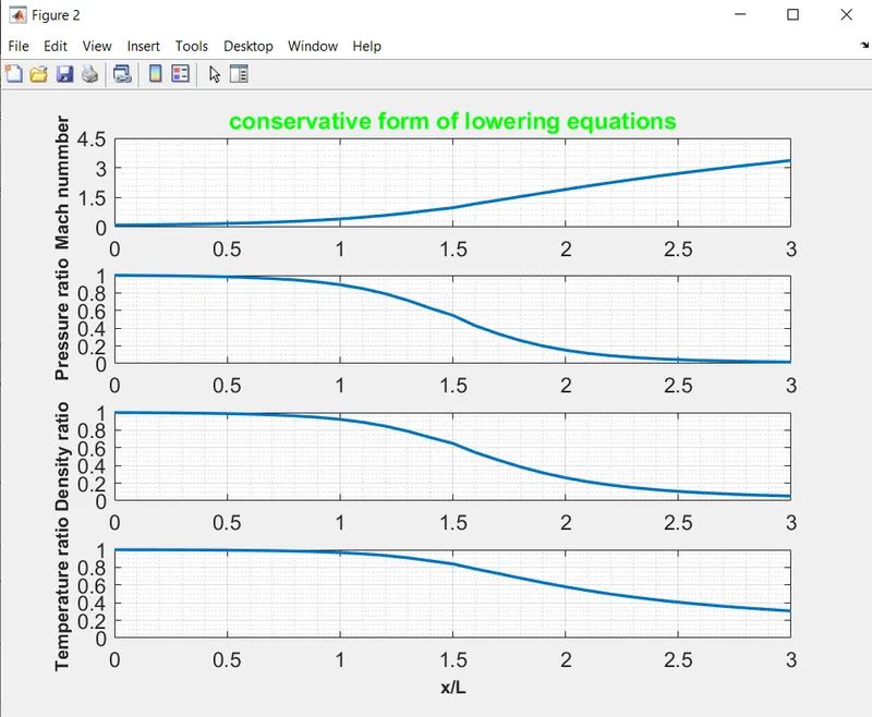
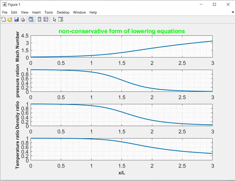
From the above two graphs, we can see that, as the Mach number increases the flow reaches from subsonic to supersonic velocity. The pressure, temperature, density shows a decline after the sonic region, till the exit of the nozzle.
Figure(3)
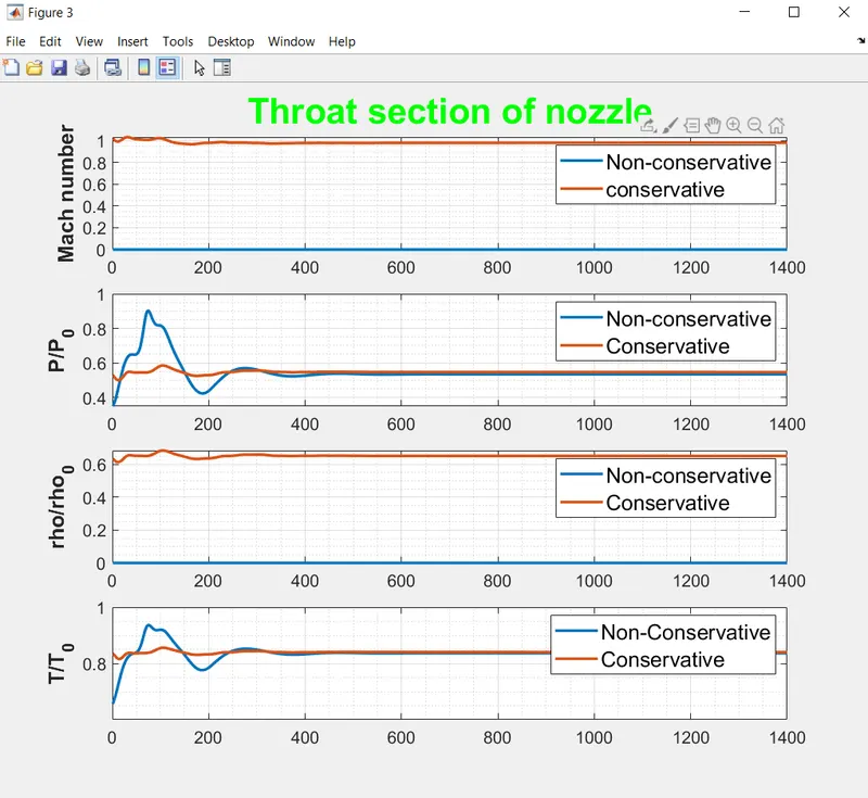
Here, we can see that the conservative form, which we used the modified initial conditions, converges to the steady-state faster than the non-conservative form.
Figure(4)
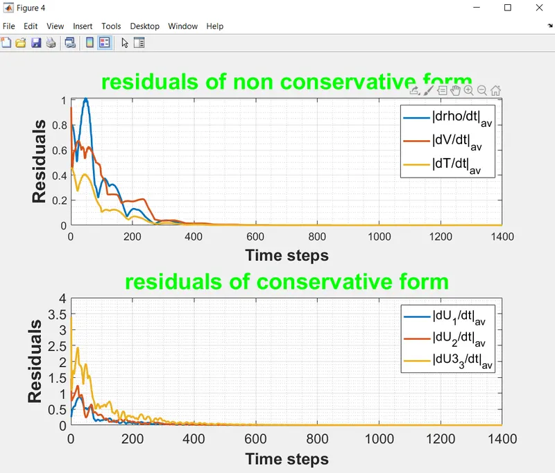
Figure(5)
Figure(6)
Figure(7)
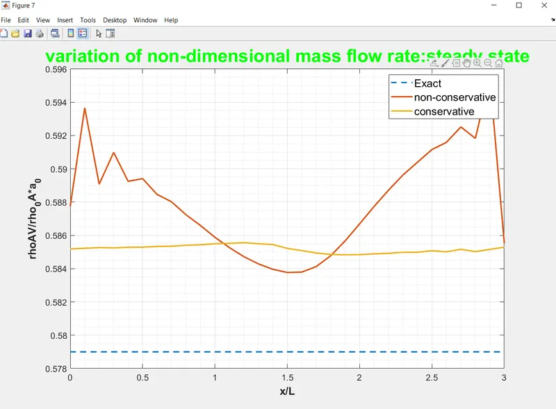
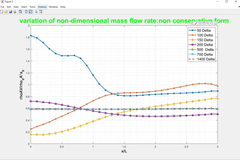
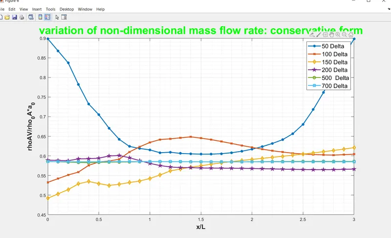
In the above graphs, we compare steady state variations of mass flow obtained with the non-conservative and conservative forms of the governing equations. Here, the steady state mass flow distribution predicted by the conservative form of the equation is much more satisfactory than that obtained from non-conservative form, on two main reasons..
1) The conservative form gives a distribution that is much closer to being a constant. In contrast, the non-conservative results have a sizable variation with some oscillations at both the inflow and outflow boundary of course on a practical basis, these variations are not apparent and the mass flow essentially appears to be constant.
2) The steady-state mass flow results obtained with the conservative form are, on the whole, much closer to the exact analytical solution
******************************************END********************************************