Week 5.1 - Mid term project - Solving the steady and unsteady 2D heat conduction problem
Solving the above-given question in both Steady-state analysis and Unsteady or Transient state analysis.
1) STEADY-STATE ANALYSIS
In this type of analysis, the tmeperature remains unchanged, that is it will not change with time.
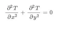
The equation for the Steady-state analysis is given by
Our defined Boundary conditions will be like this..
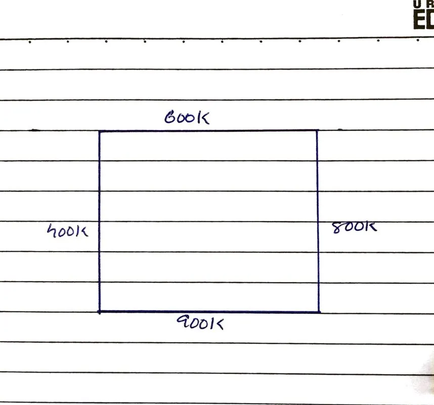
Assume that we have uniform grid points.
MATLAB PROGRAM
*** Substitute value in 49th line ,"Iterative solver", 1 = jacobi , 2 = Gauss siedel , 3 = SOR Method.***
clear all
close all
clc
%steady state 2D heat conduction equation
%d^2T/dx^2 + d^2T/dy^2 = 0
%initial conditions (assumptions)
l = 1; %length of the domain
nx = 10; %number of nodes in the x direction
ny = 10; %number of nodes in the y direction
x = linspace(0,l,nx);
y = linspace(0,l,ny);
dx = 1/(nx-1); % change of length in the x axis
dy = 1/(ny-1); %change of length in the y axis
error = 9e9;
tol = 1e-4;
%Boundary conditions as per questions
T_r = 800;
T_l =400;
T_b = 900;
T_t = 600;
T = 298*ones(nx,ny);
%relaxation factor
omega = 1.2;
% defining temperature at the boundary
T(:,1) = T_l;
T(:,end) = T_r;
T(end,:) = T_b;
T(1,:) = T_t;
%creating a copy of old T values
[X,Y] = meshgrid(x,y);
Told = T;
iterative_solver = 3;
k = 2/dx^2 + 2/dy^2;
%JACOBI METHOD
if iterative_solver == 1
jacobi_iter = 1;
while(error>tol)
for i = 2:nx-1
for j = 2:ny-1
term1 =(Told(i-1,j)+Told(i+1,j))/(k*(dx^2));
term2 =(Told(i,j-1)+Told(i,j+1))/(k*(dy^2));
T(i,j) = term1+term2;
end
end
error = max(max(abs(Told - T)));
Told = T; % updating the Told value
jacobi_iter = jacobi_iter +1;
%plotting
figure(1)
[A,B]= contourf(X,Y,T);
set(gca,'YDIR','reverse')
colorbar
colormap(jet)
clabel(A,B);
text=sprintf('Jacobi_iteration = %d',jacobi_iter);
ylabel('Y')
title(text)
pause(0.003)
end
end
%GAUS SIEDEL MEATHOD
if iterative_solver == 2
gs_iter = 1;
while(error>tol)
for i = 2:nx-1
for j = 2:ny-1
term1 =(T(i-1,j)+Told(i+1,j))/(k*(dx^2));
term2 =(T(i,j-1)+Told(i,j+1))/(k*(dy^2));
T(i,j) = term1+term2;
end
end
error = max(max(abs(Told - T)));
Told = T; % updating the Told value
gs_iter = gs_iter +1;
%plotting
figure(1)
[A,B]= contourf(X,Y,T);
set(gca,'YDIR','reverse')
colorbar
colormap(jet)
clabel(A,B);
text=sprintf('Gauss seidel iteration = %d',gs_iter);
ylabel('Y')
title(text)
pause(0.003)
end
end
% SOR METHOD
if iterative_solver == 3
sor_iter = 1;
while(error>tol)
for i = 2:nx-1
for j = 2:ny-1
term1 =(T(i-1,j)+Told(i+1,j))/(k*(dx^2));
term2 =(T(i,j-1)+Told(i,j+1))/(k*(dy^2));
T(i,j) = (1-omega)*Told(i,j)+omega*(term1+term2);
end
end
error = max(max(abs(Told - T)));
Told = T; % updating the Told value
sor_iter = sor_iter +1;
%plotting
figure(1)
[A,B]= contourf(X,Y,T);
set(gca,'YDIR','reverse')
colorbar
colormap(jet)
clabel(A,B);
text=sprintf('SOR iteration = %d',sor_iter);
ylabel('Y')
title(text)
pause(0.003)
end
end
RESULTS
1) JACOBI METHOD
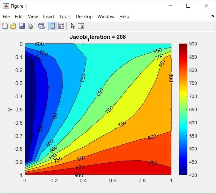
Number of Iterations = 208
Number of grids = 10
2) GAUSS SIEDEL METHOD
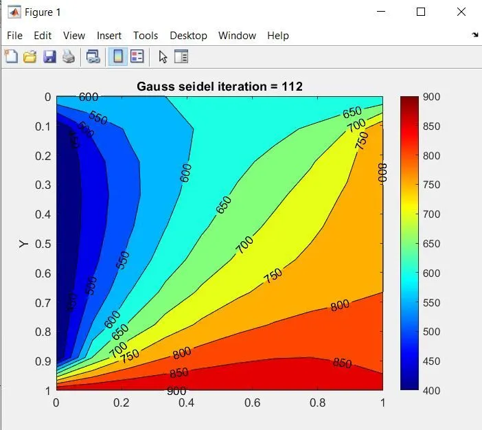
Number of Iterations = 112
Number of grid points = 10
3) SOR Method
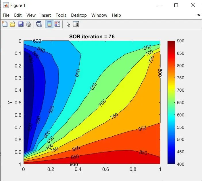
Number of Iterations = 76
Number of Grid points = 10
UNSTEADY / TRANSIENT STATE HEAT CONDUCTION ANALYSIS
The equation for Transient heat conduction is
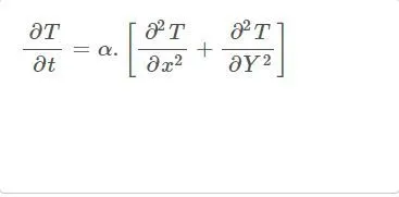
When we have a time derivative, we apply the Time marching equation... Then this equation will be
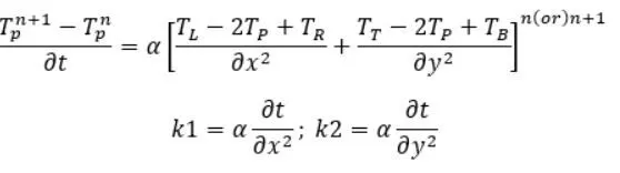
Here 'n' denotes the explicit term and 'n+1' for the implicit term.
So, the final equation derived for the explicit equation is.

and for the Implicit method is

THE MATLAB CODE FOR THE EXPLICIT METHOD IS
% EXPLICIT METHOD
clear all
close all
clc
l = 1; %length of the domain
nx = 10; %number of nodes in x direction
ny = 10; %number of nodes in y direction
x=linspace(0,l,nx);
y=linspace(0,l,ny);
dx=l/(nx-1); %change of length in x axis
dy=l/(ny-1); %change of length in y axis
dt= 0.001; %time steps
error = 9e9; %error defined
tol = 1e-4; %tolerance defined
%Temperature in each direction
T_l =400; % left
T_r =800; % right
T_t = 600; % top
T_b = 900; % bottom
% Creating an array , T matrix
T = 298*ones(nx,ny);
%assigning corresonding temp value to each directions in the matrix
T(:,1) = T_l;
T(:,end) = T_r;
T(end,:) = T_b;
T(1,:) = T_t;
% defining the BC inside the matrix
T(1,1)=(900+400)/2;
T(1,end)=(900+800)/2;
T(end,1) = (400+600)/2;
T(end,end)=(800+600)/2;
alpha = 1.4; %Diffusivity term
k1=alpha*dt/dx^2;
k2=alpha*dt/dy^2;
[X Y] = meshgrid(x,y);
%creating a copy of old T values
Told=T;
CFL = k1+k2 %CFL is a term to determine weather the soln is stable or unstable. For a stable equation CF should be less than or equal to 0.5
unsteady_explicit_iter =1;
for nt = 1:1400
while(error>tol)
for i=2:nx-1
for j=2:ny-1
term1 = Told(i-1,j)-2*Told(i,j)+Told(i+1,j);
term2 = Told(i,j-1)-2*Told(i,j)+Told(i,j+1);
T(i,j) = Told(i,j)+k1*term1+k2*term2;
end
end
error = max(max(abs(Told-T)));
Told =T;
unsteady_explicit_iter = unsteady_explicit_iter +1;
figure(1)
[A B]= contourf(X,Y,T);
set(gca,'YDIR','reverse')
colorbar
colormap(jet)
clabel(A,B);
text = sprintf('Unsteady Explicit Iterations = %d',unsteady_explicit_iter);
ylabel('y')
title(text)
%pause(0.03)
end
end
RESULTS
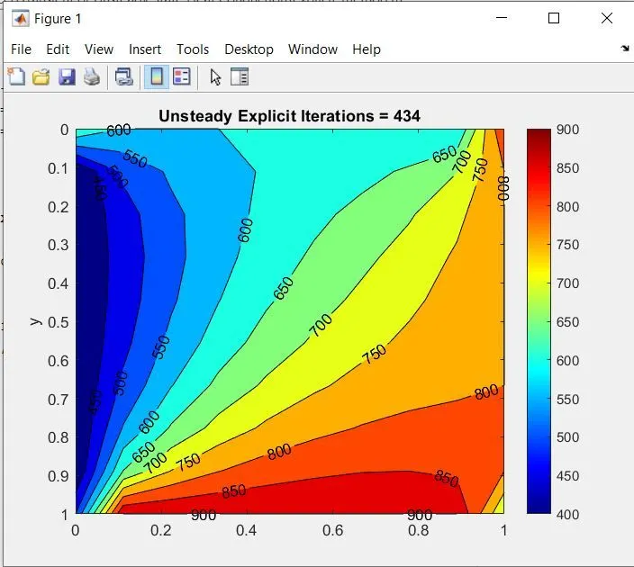
Number of Grid points = 10
Number of Iterations = 434
CFL Number = 0.2268
MATLAB PROGRAM FOR THE IMPLICIT METHOD
***Assign values on the 67 th line, for 'Iterative_solver'. 1) = Jacobi Method 2)Gauss Siedel Method
3) SOR Method
clear all
close all
clc
l = 1; %length of the domain
nx = 10; %number of nodes in x direction
ny = 10; %number of nodes in y direction
x=linspace(0,l,nx);
y=linspace(0,l,ny);
dx=1/(nx-1); %change of length in x axis
dy=1/(ny-1); %change of length in y axis
dt= 0.001; %time steps
error = 9e9; %error defined
tol = 1e-4; %tolerance defined
%Temperature in each direction
T_l =400; % left
T_r =800; % right
T_t = 600; % top
T_b = 900; % bottom
% Creating an array , T matrix
T = 298*ones(nx,ny);
%assigning corresonding temp value to each directions in the matrix
T(:,1) = T_l;
T(:,end) = T_r;
T(end,:) = T_b;
T(1,:) = T_t;
% defining the BC inside the matrix
T(1,1)=(900+400)/2;
T(1,end)=(900+800)/2;
T(end,1) = (400+600)/2;
T(end,end)=(800+600)/2;
alpha = 1.4; %Diffusivity term
k1=alpha*dt/dx^2;
k2=alpha*dt/dy^2;
[X Y] = meshgrid(x,y);
%creating a copy of old T values
%Told=T;
CFL = k1+k2 %CFL is a term to determine weather the soln is stable or unstable. For a stable equation CF should be less than or equal to 0.5
Told = T;
T_prev_dt = T;
iter = 1;
omega = 1.1;
iterative_solver =3
for nt = 1:1400
%Jacobi Method
if iterative_solver ==1
term1=(1+2*k1+2*k2)^(-1);
term2 = k1*term1;
term3 = k2*term1;
error = 9e9;
while(error>tol)
for i=2:nx-1
for j=2:ny-1
H = (Told(i-1,j)+Told(i+1,j));
V = (Told(i,j-1)+Told(i,j+1));
T(i,j) = (T_prev_dt(i,j)*term1)+(H*term2)+(V*term3);
end
end
error = max(max(abs(Told-T)));
Told =T;
iter = iter+1;
end
end
%Gauss Seidel Method
if iterative_solver ==2
term1=(1+2*k1+2*k2)^(-1);
term2 = k1*term1;
term3 = k2*term1;
error = 9e9;
while(error>tol)
for i=2:nx-1
for j=2:ny-1
H = (T(i-1,j)+Told(i+1,j));
V = (T(i,j-1)+Told(i,j+1));
T(i,j) = (T_prev_dt(i,j)*term1)+(H*term2)+(V*term3);
end
end
error = max(max(abs(Told-T)));
Told =T;
iter = iter+1;
end
end
%SOR Method
if iterative_solver ==3
term1=(1+2*k1+2*k2)^(-1);
term2 = k1*term1;
term3 = k2*term1;
error = 9e9;
while(error>tol)
for i=2:nx-1
for j=2:ny-1
H = (T(i-1,j)+Told(i+1,j));
V = (T(i,j-1)+Told(i,j+1));
T(i,j) = (1-omega)*Told(i,j)+omega*((T_prev_dt(i,j)*term1)+(H*term2)+(V*term3));
end
end
error = max(max(abs(Told-T)));
Told =T;
iter = iter+1;
end
end
T_prev_dt = T;
end
figure(1)
[P Q]= contourf(X,Y,T);
set(gca,'YDIR','reverse')
colorbar
colormap(jet)
clabel(P,Q);
text = sprintf('Implicit Iterations= %d',iter);
ylabel('y')
title(text)
pause(0.0003)
RESULTS
Number of Iterations = 3669
CFL Number = 0.2268
2) GAUSS SIEDEL METHOD
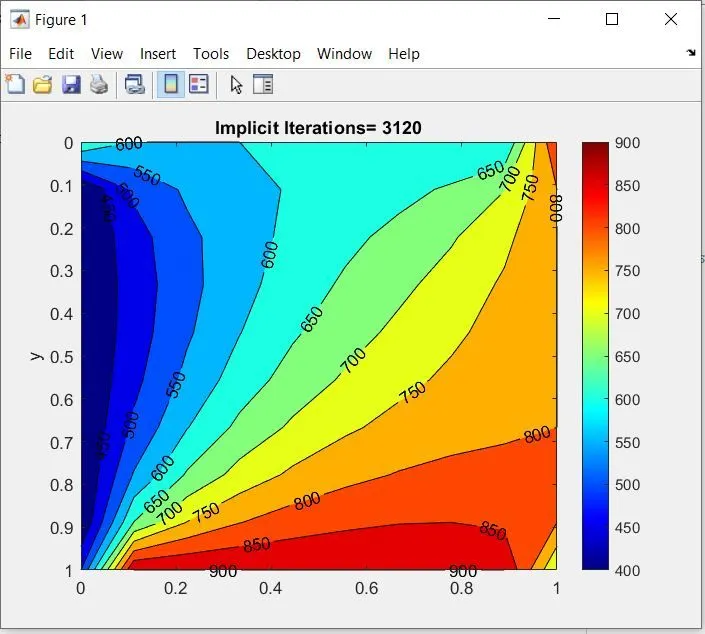
Number of Grid points = 10
Number of Iterations = 3120
CFL Number = 0.2268
3) SOR METHOD
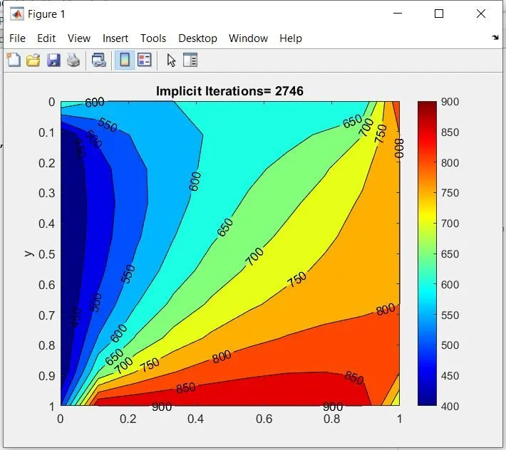
Number of Grid points = 10
Number of Iterations = 2746
CFL Number = 0.2268
OBSERVATIONS
- The result of the steady-state heat conduction narrows in few iterations
- The unsteady-state heat conduction takes a lot of time for calculation because its a function of both position and time while the steady-state is only a function of time.
- SOR gives fast results.