Week 8- Moving zones approach in Fluent

Moving zones approach in Fluent

Aim: To simulate rotary motion using moving mesh.

Objective:

1. What are the approaches by which you would model moving zones?
2. Which approach would you use to model unsteady phenomena?
3. Simulate rotary motion for the geometry give and plot the velocity profile of the fluid motion

Theory:

There are two approaches to model rotary motion

1. Moving reference frame

2. Moving mesh appraoch.

Moving refernce frame:

A Moving Reference Frame is a relatively simple, robust, and efficient steady-state, Computational fluid dynamics modeling technique to simulate rotating machinery.

The principal reason for employing a moving reference frame is to render a problem which is unsteady in the stationary frame steady with respect to the moving frame. For a steadily rotating frame it is possible to transform the equations of fluid motion to the rotating frame such that steady-state solutions. If the rotational speed is not constant, the transformed equations will contain additional terms which are not included in fluent formulation, while unsteady simulations can be studied in moving refernce frame with constant rotational speed.

Other way to compute a flow field that can be used as an initial condition for a transient sliding mesh calculation.

There are two types of moving refernce frame approach

1. Single moving refrence frame.

2. Multiple moving refernce frame that uses a mixing plane approach.

Moving Mesh approach:

Moving mesh approach is used to model unstaedy flows. Generally flows with vortex induced and for the flows for inetraction of vortex with the bodies. When a time-accurate solution for rotor-stator interaction is desired, you must use the sliding mesh model to compute the unsteady flow field

Two types of mesh is possible:

1. Conformal Mesh - The node at each sides of rotating frames are perfectly alligned.

2. Non-Conformal Mesh - The node at each sides of rotating frames are not perfectly alligned.

Procedure:

Import the mesh file in fluent.

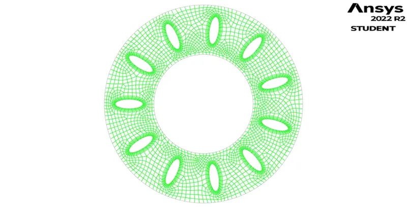
Setup:

Solver - Pressure based.

Steady state.

Viscous: Realizable K-epsilon.

Material : Air.

Angular velocity: 250 rpm.

Wall : Moving ( Rotational)

Hybrid Initialization.

Courant number = 10

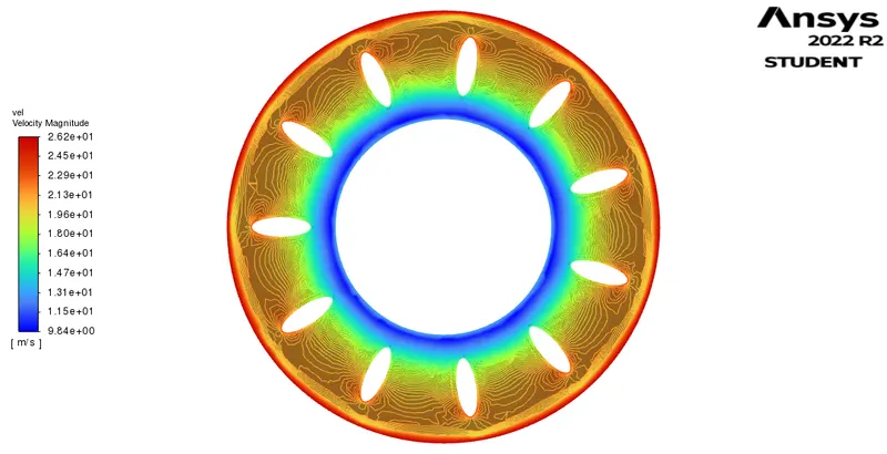
Velocity contour:

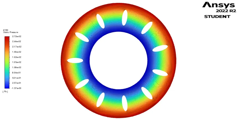
Pressure contour:

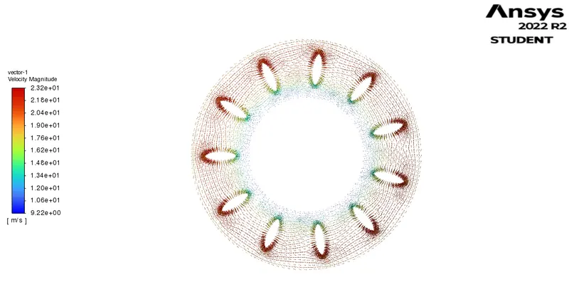
Velocity vector profile:

Conclusion:

Outer maximum velocity is 232 m/s.

Moving frame and moving mesh is explained.