Week 7 - Simulation of a 1D Super-sonic nozzle flow simulation using Macormack Method
MacCormack's technique to solve conservation and non-conservation forms of the governing equations
Aim: To solve conservation and non-conservation forms of the governing equations and using the MacCormack's technique.
Objective: To find the following,
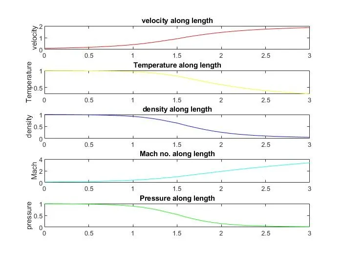
1. Steady-state distribution of primitive variables inside the nozzle
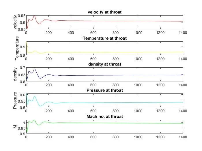
2. Time-wise variation of the primitive variables
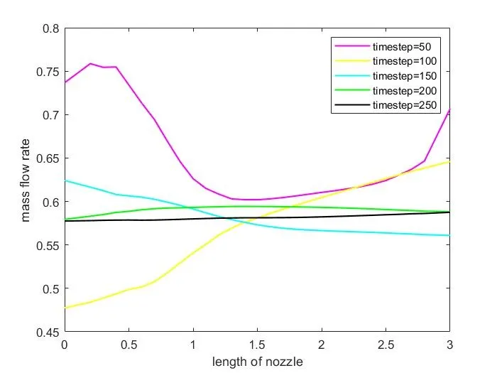
3. Variation of Mass flow rate distribution inside the nozzle at different time steps during the time-marching process
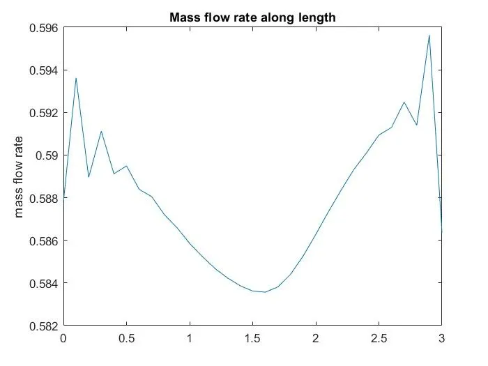
4. Comparison of Normalized mass flow rate distributions of both forms
Solution:
Nozzle:
Let the Isentropic flow through the convergent divergent nozzle is assumed to be 1D quasi state. The simulation by using the MacCormark's method. It is discretization scheme used for solution of PDEs.
Flow is accelerated by the pressure ratio in the nozzle `p_0/p_e`.
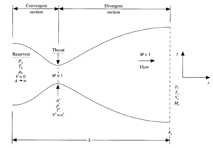
Whereas convergent part is subsonic (M<1) and divergent part is supersonic(M>1), at throat M=1.
P=Pressure
T=Temperature
`rho`=density
V= velocity
M= Mach number
In MacCormark's method the governing equations are modelled into two forms:
1. Conservative form
2. Non conservative form
Non dimensional primitive variable are found using equaitons in these 2 forms,
Non conservative form:
Equations involved are mentioned in the form of PDE,
continuity equation:
`(drho')/dt= rho'(dV')/(dx')-rho'V'(d(lnA))/(dx')-V'(dp')/(dx')`
momentum equation:
`(dV')/dt= V'(dV')/(dx')-(1/gamma)((dT')/(dx')+((T')/(rho')+(dp')/(dx')))`
energy equation:
`(dT')/dt= V'(dT')/(dx')-(gamma-1)(T')((dV')/(dx')+(V'((d(lnA'))/(dx')))`
Conservative form:
Equations involved are mentioned in the form of PDE
Continuity equation:
`(drho'A')/dt+(drho'A'V')/dx=0`
Momentum equation:
`(drho'A'V')/dt+(d(rho'A'V'^2+(1/gamma)p'A'))/dx=(1/gamma)p'(dA')/(dx)`
Energy equaiton:
`d(rho'(((T')/(gamma-1))+((gamma)/2(V'^2)A'))/(dt))+d(rho'((T')/(gamma-1))+((gamma)/2(V'^2)A'V'+(p'A'V')))/(dx')=0`
First term in the equations are mentioned as U1,U2,U3 and other as flux terms F1, F2, F3.
Above mentioned equations are used to find the solutions
MacCarmark method:
In this method to discretize the solution two step Lax-Wendroff scheme is applied.
The method is proceeded in 2 steps, predictor and corrector step followed to find average of the in final step.
1. Predictor step: In this step value of u at time n+1 is obtained to by replacing the spatial derivative in prevoious order using Forward difference scheme.
At given time time t primitive variable are calculated
At intermediate step we find the primitive variable value at time t+dt,
2. Corrector step: In this step predicted value is corrected using Backward difference scheme of spacial derivative.
Then the average of both values are taken to find the solution.
Matlab colde for non-conservative method :
clear all
close all
clc


n=31;
x=linspace(0,3,n); %length=3
dx=x(2)-x(1);
gamma=1.4;


%cal initial prop
%density
rho=1-0.316.*x;
%Temperature
T=1-0.2314.*x;
%velocity
v=(0.1+1.09*x).*T.^0.5;
% area
A=1+2.2*(x-1.5).^2;
%velocity of sound
a=sqrt(T);
CFL=0.4;

%time steps
nt=1400;
%dt=0.001;
dt=min(CFL.*dx./(a+v));


%outer time loop
for k=1:nt

    %predictor step
    %continuity step

    rho_old=rho;
    v_old=v;
    T_old=T;

    for j=2:n-1

        dvdx=(v(j+1)-v(j))/dx;
        drhodx=(rho(j+1)-rho(j))/dx;
        dTdx=(T(j+1)-T(j))/dx;
        dlogAdx=(log(A(j+1))-log(A(j)))/dx;

        %eqn

        drhodt_p(j)=-rho(j)*dvdx-rho(j)*v(j)*dlogAdx-v(j)*drhodx;

        %momen eqn

        dvdt_p(j)=-v(j)*dvdx-(1/gamma)* (dTdx+(T(j)/rho(j))*drhodx);

        %energy eqn
        dTdt_p(j)=-v(j)*dTdx-(gamma-1)*T(j)*((dvdx)+v(j)*dlogAdx);


        %soln update
        %intermediate step
        rho(j)=rho(j)+drhodt_p(j)*dt;
        v(j)=v(j)+dvdt_p(j)*dt;
        T(j)= T(j)+ dTdt_p(j)*dt;


    end


    %correc step
    for j=2:n-1

        dvdx=(v(j)-v(j-1))/dx;
        drhodx=(rho(j)-rho(j-1))/dx;
        dTdx=(T(j)-T(j-1))/dx;
        dlogAdx=(log(A(j))-log(A(j-1)))/dx;

        %eqn

        drhodt_c(j)=-rho(j)*dvdx-rho(j)*v(j)*dlogAdx-v(j)*drhodx;

        %momen eqn

        dvdt_c(j)=-v(j)*dvdx-(1/gamma)*(dTdx+(T(j)/rho(j))*drhodx);

        %energy eqn
        dTdt_c(j)=-v(j)*dTdx-(gamma-1)*T(j)*((dvdx)+v(j)*dlogAdx);


    end

    %compute avg time der


    drhodt_avg=0.5*(drhodt_c+drhodt_p);
    dvdt_avg=0.5*(dvdt_c+dvdt_p);
    dTdt_avg=0.5*(dTdt_c+dTdt_p);

    %final values update

    for i=2:n-1

        rho(i)=rho_old(i)+drhodt_avg(i)*dt;
        v(i)=v_old(i)+dvdt_avg(i)*dt;
        T(i)=T_old(i)+dTdt_avg(i)*dt;
    end

    %BC
    %inlet

    rho(1)=1;
    T(1)=1;
    v(1)=2*v(2)-v(3);

    %outlet

    v(n)=2*v(n-1)-v(n-2);
    rho(n)=2*rho(n-1)-rho(n-2);
    T(n)=2*T(n-1)-T(n-2);
    %mach no.
    M=v./sqrt(T);
    %pressure
    P=rho.*T;
    %mass flow rate

    mfr= rho.*v.*A;

    % values at throat section
    throat=(A==1);
    rho_throat(k)=rho(throat);
    T_throat(k)=T(throat);
    v_throat(k)=v(throat);
    mfr_throat(k)=mfr(throat);
    P_throat(k)=rho_throat(k).*T_throat(k);
    M_throat(k)=v_throat(k)./sqrt(T_throat(k));


    figure(3)

    if k==50
        plot(x,mfr,'m','linewidth',1.25,'displayName',['timestep=',num2str(k)])
        hold on
    elseif k==100
        plot(x,mfr,'y','linewidth',1.25,'displayName',['timestep=',num2str(k)])
        hold on
    elseif k==150
        plot(x,mfr,'c','linewidth',1.25,'displayName',['timestep=',num2str(k)])
        hold on
    elseif k==200
        plot(x,mfr,'g','linewidth',1.25,'displayName',['timestep=',num2str(k)])
        hold on
    elseif k==250
        plot(x,mfr,'k','linewidth',1.25,'displayName',['timestep=',num2str(k)])
        hold on
    end
    xlabel('length of nozzle')
    ylabel('mass flow rate')
    legend

end
figure(1)
subplot(5,1,1)
plot(x,v,'r')
title('velocity along length')
ylabel('velocity')

subplot(5,1,2)
plot(x,T,'y')
title('Temperature along length')
ylabel('Temperature')

subplot(5,1,3)
plot(x,rho,'b')
title('density along length')
ylabel('density')

subplot(5,1,4)
plot(x,M,'c')
title('Mach no. along length')
ylabel('Mach')

subplot(5,1,5)
plot(x,P,'g')
title('Pressure along length')
ylabel('pressure')


figure(2)
plot(x,mfr)
title('Mass flow rate along length')
ylabel('mass flow rate')

figure(4)
subplot(5,1,1)

plot(v_throat,'r')
title('velocity at throat')
ylabel('velocity')
% pause(0.1)
subplot(5,1,2)
plot(T_throat,'y')
title('Temperature at throat')
ylabel('Temperature')

subplot(5,1,3)
plot(rho_throat,'b')
title('density at throat')
ylabel('density')

subplot(5,1,4)
plot(P_throat,'c')
title('Pressure at throat')
ylabel('Pressure')

subplot(5,1,5)
plot(M_throat,'g')
title('Mach no. at throat')
ylabel('M')
Explaination:
1. Initialize the variables `rho`,V, T, A.
2. Minimum of dt values is calculated.
3. Computing the predicter step time derivatives for `rho`,V, T.
4. Updating all the values in loop.
5. Computing the correcter step time derivative for updated values of `rho`,V, T.
6. Updating all the values in loop.
7. To compute the average of the predictor and corrector step values.
8. Applying boundary conditions.
9. Plotting the graph.
Matlab code for conservative method:
clear all
close all
clc


n=31;
x=linspace(0,3,n);
dx=x(2)-x(1);
gamma=1.4;

for i=1:n
    if (x(i)>=0 && x(i)<=0.5)
        rho_con(i)=1;
        T_con(i)=1;
    elseif (x(i)>=0.5 && x(i)<=1.5)
        rho_con(i)=1- 0.366*(x(i)-0.5);
        T_con(i)=1-0.167*(x(i)-0.5);
    elseif (x(i)>=1.5 && x(i)<=3)
        rho_con(i)=0.634-0.3879*(x(i)-1.5);
        T_con(i)=0.833-0.3507*(x(i)-1.5);
    end
end

%initial values

%speed of sound
a=sqrt(T_con);


%pressure
P_con=rho_con.*T_con;
% area
A=1+2.2*(x-1.5).^2;
%velocity
v_con=0.59./(rho_con.*A);


CFL=0.7;

%   initial solution vectors
u1=rho_con.*A;
u2=rho_con.*A.*v_con;
u3=rho_con.*A.*(T_con./(gamma-1))+((gamma/2).*v_con.^2);


%time steps
nt=1400;


%outer time loop
for k=1:nt

    dt=min(CFL.*dx./(a+v_con));
% dt=0.0161


    %continuity step

    u1_old=u1;
    u2_old=u2;
    u3_old=u3;

    % flux vector
    F1=u2;
    F2=((u2.^2)./u1)+((gamma-1)/gamma)*(u3-(gamma/2)*((u2.^2)./u1));
    F3=((gamma*u2.*u3)./u1)-(gamma*0.5*(gamma-1)*(u2.^3)./(u1.^2));


% predictor step
    for j=2:n-1

        %calc
        J2(j)=(1/gamma)*(rho_con(j)*T_con(j))*(A(j+1)-A(j))/dx;


        % continuity eqn

        du1_dt_p(j)=-(F1(j+1)-F1(j))/dx;

        %momen eqn

        du2_dt_p(j)=-((F2(j+1)-F2(j))/dx)+J2(j);

        %energy eqn
        du3_dt_p(j)=-((F3(j+1)-F3(j))/dx);


        %soln update

      u1(j)=u1(j)+du1_dt_p(j)*dt;
      u2(j)=u2(j)+du2_dt_p(j)*dt;
      u3(j)=u3(j)+du3_dt_p(j)*dt;

    end

    rho_con=u1./A;
    v_con=u2./u1;
    T_con=(gamma-1)*((u3./u1-(gamma/2)*(v_con).^2));


    %updating flux

    F1=u2;
    F2=((u2.^2)./u1)+((gamma-1)/gamma)*(u3-(gamma/2)*((u2.^2)./u1));
    F3=((gamma*u2.*u3)./u1)-(gamma*(gamma-1)*((u2.^3)./(2*u1.^2)));


    %correc step
    for j=2:n-1

        %source term
        J2(j)=(1/gamma)*rho_con(j)*T_con(j)*(A(j)-A(j-1))/dx;


%simplifying
du1_dt_c(j)=-((F1(j)-F1(j-1))/dx);
du2_dt_c(j)=-((F2(j)-F2(j-1))/dx)+J2(j);
du3_dt_c(j)=-((F3(j)-F3(j-1))/dx);


    end

    %compute avg time der


    du1_dt_avg=0.5.*(du1_dt_p+du1_dt_c);
    du2_dt_avg=0.5.*(du2_dt_p+du2_dt_c);
    du3_dt_avg=0.5.*(du3_dt_p+du3_dt_c)


    %final values update

    for i=2:n-1

        u1(i)=u1_old(i)+du1_dt_avg(i)*dt;
        u2(i)=u2_old(i)+du2_dt_avg(i)*dt;
        u3(i)=u3_old(i)+du3_dt_avg(i)*dt;
    end

    %BC
    %inlet

    u1(1)=rho_con(1)*A(1);
    u2(1)=2*u2(2)-u2(3);
    v_con(1)=u2(1)./u1(1);
    u3(1)=u1(1)*((T_con(1)/(gamma-1))+(0.5*gamma*(v_con(1)).^2));


    %outlet

    u1(n)=2*u1(n-1)-u1(n-2);
    u2(n)=2*u2(n-1)-u2(n-2);
    u3(n)=2*u3(n-1)-u3(n-2);

        % primitive variable


    rho_con=u1./A;
    v_con=u2./u1;
    T_con=(gamma-1)*((u3./u1-(gamma/2)*(v_con).^2));


    %mach no.
    M=(v_con./sqrt(T_con));
    %pressure
    P_con=rho_con.*T_con;


    %mass flow rate

    mfr_con= rho_con.*v_con.*A;


    % values at throat section
    throat=(A==1);
    rho_throat(k)=rho_con(throat);
    T_throat(k)=T_con(throat);
    v_throat(k)=v_con(throat);
    mfr_throat(k)=mfr_con(throat);
    P_throat(k)=rho_throat(k).*T_throat(k);
    M_throat(k)=v_throat(k)./sqrt(T_throat(k));


    figure(1)

    if k==50
        plot(x,mfr_con,'m','linewidth',1.25,'displayName',['timestep=',num2str(k)])
        hold on
    elseif k==100
        plot(x,mfr_con,'y','linewidth',1.25,'displayName',['timestep=',num2str(k)])
        hold on
    elseif k==150
        plot(x,mfr_con,'c','linewidth',1.25,'displayName',['timestep=',num2str(k)])
        hold on
    elseif k==200
        plot(x,mfr_con,'g','linewidth',1.25,'displayName',['timestep=',num2str(k)])
        hold on
    elseif k==250
        plot(x,mfr_con,'k','linewidth',1.25,'displayName',['timestep=',num2str(k)])
        hold on
    end
    xlabel('length of nozzle')
    ylabel('mass flow rate')
    legend

end
figure(2)
subplot(5,1,1)

plot(x,v_con,'r')
title('velocity along length')
ylabel('velocity')

subplot(5,1,2)
plot(x,T_con,'y')
title('Temperature along length')
ylabel('Temperature')

subplot(5,1,3)
plot(x,rho_con,'b')
title('density along length')
ylabel('density')

subplot(5,1,4)
plot(x,M,'c')
title('Mach no. along length')
ylabel('Mach')

subplot(5,1,5)
plot(x,P_con,'g')
title('Pressure along length')
ylabel('pressure')


figure(3)
plot(x,mfr_con)
title('Mass flow rate along length')
ylabel('mass flow rate')
axis([0 3,0.582 0.596]) %To compare with non conservative method

figure(4)
subplot(5,1,1)

plot(v_throat,'r')
title('velocity at throat')
ylabel('velocity')
% pause(0.1)
subplot(5,1,2)
plot(T_throat,'y')
title('Temperature at throat')
ylabel('Temperature')

subplot(5,1,3)
plot(rho_throat,'b')
title('density at throat')
ylabel('density')

subplot(5,1,4)
plot(P_throat,'c')
title('Pressure at throat')
ylabel('Pressure')

subplot(5,1,5)
plot(M_throat,'g')
title('Mach no. at throat')
ylabel('M')
Explaination:
1. Initial conditions are applied, for A
a. And for `rho`,T for different values of x.
b. Also V
2. Solution variables are initialized.
3. Adaptive time step is obtained by taking minimum of dt.
4. Computing the flux terms by forward difference scheme in spacial derivative.
5. Obtaining the time derivaitve of U values from flux terms, and calculate J2 term.
6. Updating the valus of U1, U2, U3.
7. Computing `rho`,V, T, from U terms.
8. To get intermediate solution by predictor and old values.
9. Re-compute the values of Flux terms.
10. Obtaining the time derivative terms of U terms using flux terms by Backward differencing.
11. Compute the average of primitive variable obtained from both steps.
12. Update the U terms with average variables.
13. Applying Boundary conditons for inlet and outlet.
14. Re-compute the values of `rho`,V, T from upadted U terms.
Plotting the graph:
Non conservative method:
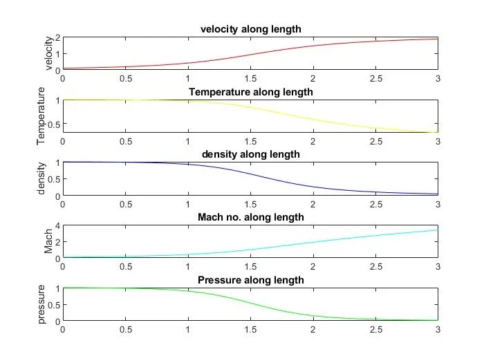
1. Steady-state variation of Primitive variable inside the nozzle.
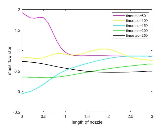
2. Mass flow rate at different time steps during the time-marching process:
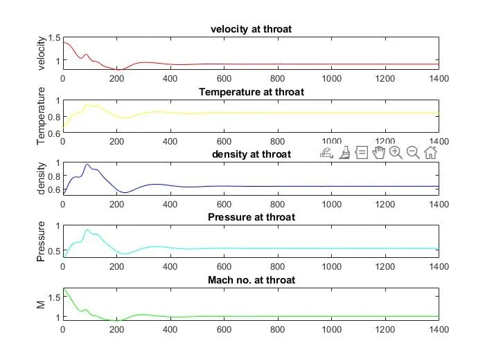
3. Time-wise variation of the primitive variables at throat:
Conservative method:
1. Steady-state variation of Primitive variable inside the nozzle:
2. Mass flow rate at different time steps during the time-marching process:
3. Time-wise variation of the primitive variables at throat:
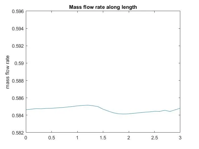
4. Comparison of Normalized mass flow rate distributions of both forms:
a. Non conservative forms:
b. Conservative form
Conclusion:
1. In both, conservative and non conservative form, velocity and Mach no. increases in subsonic of convergent section, whereas temperature, pressure and density decreases along length.
2. In non conservative solution at throat :density, pressure, temperature initially increases as time progress and decreases upto 200 th step, whereas velocity decreases. After that these values becomes stable gradually
In conservative solution at throat: density, pressure, temperature initially increases gradually and decreases upto 200 th step, whereas velocity decreases. After that these values becomes stable gradually. But in this case variation is less compared to other.
3. Normalized mass flow rate:
The variation of mass flow rate in non conservative form is more than conservative form. (In conservative form it is more stable.)
4. Mass flow rate at different time steps: In both form mass flow rate becomes gradually stable at higher time steps.