Week 3.5 - Deriving 4th order approximation of a 2nd order derivative using Taylor Table method

Deriving 4th order approximation of a 2nd order derivative using Taylor Table method

Aim: To derive the following 4th order approximations of the second-order derivative.

1. Central difference

2. Skewed right-sided difference

3. Skewed left-sided difference

and write Matlab code for the above.

Objective:

To write a program in Matlab to evaluate the second-order derivative of the analytical function exp(x)*cos(x) and compare it with the 3 numerical approximations derived.

To plot and compare the absolute error between the above-mentioned schemes

Solution:

Fourth order approximation for 2nd order derivative can be solved by following methods, using taylor table

Derivations:

1. Central difference:

no. of points=5, 2 points to left and 2 points to right of i

Second order derivative can be written as

`(del^2u)/(delx^2)=af(i-2)+bf(i-1)+cf(i)+df(i+1)+ef(i+2)`

N=P-Q+1= 5-2+1= 4

fourth order derivative

	f(i)	`dx(delf)/(delx)`	`dx^2(del^2f)/(delx^2)`	`dx^3(del^3f)/(delx^3)`	`dx^4(del^4f)/(delx^4)`	`dx^5(del^5f)/(delx^5)`	`dx^6(del^6f)/(delx^6)`
af(i-1)	a	-2a	4/2! a	-8/3! a	16/4! a	-32/5! a	64/6! a
bf(i-2)	b	-b	b/2!	-b/3!	b/4!	-b/5!	b/6!
cf(i)	c	0	0	0	0	0	0
df(i+1)	d	d	d/2!	d/3!	d/4!	d/5!	d/6!
ef(i+2)	e	2e	4e/2!	8e/3!	16e/4!	32e/5!	64e/6!
sum	0	0	1	0	0	0

Solving in matrix form:

A=[ 1.0000 1.0000 1.0000 1.0000 1.0000
-2.0000 -1.0000 0 1.0000 2.0000
2.0000 0.5000 0 0.5000 2.0000
-1.3300 -0.1667 0 0.1667 1.3300
0.6670 0.0417 0 0.0417 0.6670 ]

X=[a;b;c;d;e;g]

B=[0;0;1;0;0]

Solving for co-effecients

a=-0.0834
b=1.3335
c=-2.5002
d=1.3335
e=-0.0834

2. Skewed right sided difference:

no. of points=5, 5 points to right of i

Second order derivative can be written as

`(del^2u)/(delx^2)=af(i)+bf(i+1)+cf(i+2)+df(i+3)+ef(i+4)+gf(i+5)`

P= N-Q= 6-2 =4

fourth order approximation

taylor table method:

	f(i)	`dx(delf)/(delx)`	`dx^2(del^2f)/(delx^2)`	`dx^3(del^3f)/(delx^3)`	`dx^4(del^4f)/(delx^4)`	`dx^5(del^5f)/(delx^5)`	`dx^6(del^6f)/(delx^6)`
af(i)	a	0	0	0	0	0	0
bf(i+1)	b	b	b/2!	b/3!	b/4!	b/5!	b/6!
cf(i+2)	c	2c	4c/2!	8c/3!	16c/4!	32c/5!	64c/6!
df(i+3)	d	3d	9d/2!	27d/3!	81d/4!	243d/5!	729d/6!
ef(i+4)	e	4e	16e/2!	64e/3!	256e/4!	1024e/5!	4096e/6!
gf(i+5)	g	5g	25g/2!	125g/3!	625g/4!	3125g/5!	15625g/6!
sum	0	0	1	0	0	0

Solving the equations in matrix form:

A=[ 1 1.0000 1.0000 1.0000 1.0000 1.0000
0 1.0000 2.0000 3.0000 4.0000 5.0000
0 0.5000 2.0000 4.5000 8.0000 12.5000
0 0.1667 1.3330 4.5000 10.6670 20.8330
0 0.0417 0.6670 3.3750 10.6670 26.0417
0 0.0830 0.2667 2.0250 8.5330 26.0417 ]

X=[a;b;c;d;e;g]

B=[0;0;1;0;0;0]

Solving for X,

X=`A^-1*B`

we get values for

a=3.0328
b=-9.2626
c=10.7194
d=-5.9102
e=1.5489
g=-0.1282

These co-effecients can give the value of function.

3. Skewed left sided difference method:

5 points to the left side of i

`(del^2u)/(delx^2)=af(i-5)+bf(i-4)+cf(i-3)+df(i-2)+ef(i-1)+gf(i)`

	f(i)	`dx(delf)/(delx)`	`dx^2(del^2f)/(delx^2)`	`dx^3(del^3f)/(delx^3)`	`dx^4(del^4f)/(delx^4)`	`dx^5(del^5f)/(delx^5)`	`dx^6(del^6f)/(delx^6)`
af(i)	a	-5a	25a/2!	-125a/3!	625a/4!	-3125a/5!	15625a/6!
bf(i+1)	b	-4b	16b/2!	-64b/3!	256b/4!	-1024b/5!	4096b/6!
cf(i+2)	c	-3c	9c/2!	-27c/3!	81c/4!	-243c/5!	729c/6!
df(i+3)	d	-2d	4d/2!	-8d/3!	16d/4!	-32d/5!	64d/4!
ef(i+4)	e	-e	e/2!	-e/3!	e/4!	-e/5!	e/6!
gf(i+5)	g	0	0	0	0	0	0
sum	0	0	1	0	0	0

Solving in matrix form:

A =

[1.0000 1.0000 1.0000 1.0000 1.0000 1.0000
-5.0000 -4.0000 -3.0000 -2.0000 -1.0000 0
12.5000 8.0000 4.5000 2.0000 0.5000 0
-20.8333 -10.6670 -4.5000 2.0000 0.5000 0
26.0417 10.6670 3.3750 0.6670 0.0417 0
-26.0417 -8.5330 -2.0250 -0.2667 -0.0083 0 ]

X=[a;b;c;d;e;g]

B=[0;0;1;0;0;0]

Solving for X,

X=`A^-1*B`

we get values for

a=0.1842
b=-0.8771
c=1.2480
d=0.6764
e=-2.5094
g=1.2779

Matlab code:

Let function be `f(x)=e^x*cos(x)`

analytical derivative is `-2e^x*sin(x)`

1. Central differencing function:

function out= central_difference(x,dx)

%f(x)=exp(x)*cos(x)
%taking the values from the derivation


A=[1 1 1 1 1;-2 -1 0 1 2;2 0.5 0 0.5 2;-1.33 -0.1667 0 0.1667 1.33;0.667 0.0417 0 0.0417 0.667];
B=[0;0;1;0;0];
X=inv(A)*B;

%anlaytical 2nd order derivative
analytical_derivative=-2*exp(x)*sin(x);

%error_calculation
central_difference=(X(1)*exp(x-2*dx)*cos(x-2*dx)+X(2)*exp(x-dx)*cos(x-dx)+X(3)*exp(x)*cos(x)+X(4)*exp(x+dx)*cos(x+dx)+X(5)*exp(x+2*dx)*cos(x+2*dx))/(dx^2);
out=abs(central_difference-analytical_derivative);

end

2. Right sided skewed function:

Considering the 5 points, i and 4 points right side to i

function out=right_sided_skewed(x,dx);

%f(x)=exp(x)*cos(x)
%taking the values from the derivation


A=[1 1 1 1 1;0 1 2 3 4;0 1/2 4/2 9/2 16/2;0 1/6 8/6 27/6 64/6;0 1/24 16/24 81/24 256/24];
B=[0;0;1;0;0];
X=inv(A)*B;

%anlaytical 2nd order derivative
analytical_derivative= -2*exp(x)*sin(x);

%error calculation
right_sided_skewed=(X(1)*exp(x)*cos(x)+X(2)*exp(x+dx)*cos(x+dx)+X(3)*exp(x+2*dx)*cos(x+2*dx)+X(4)*exp(x+3*dx)*cos(x+3*dx)+X(5)*exp(x+4*dx)*cos(x+4*dx))/(dx^2);

out=abs(right_sided_skewed-analytical_derivative);

end

3. Left sided skewed function:

Considering 5 points, i and 4 points to left of i

function out=left_sided_skewed(x,dx)

%f(x)=exp(x)*cos(x)
%taking the values from the derivation


A=[1 1 1 1 1;0 -1 -2 -3 -4;0 1/2 4/2 9/2 16/2;0 -1/6 -8/6 -27/6 -64/6;0 1/24 16/24 81/24 256/24];
B=[0;0;1;0;0];
X=inv(A)*B;

%anlaytical 2nd order derivative
analytical_derivative= -2*exp(x)*sin(x);

%error_calculation
left_sided_skewed=(X(5)*exp(x-4*dx)*cos(x-4*dx)+X(4)*exp(x-3*dx)*cos(x-3*dx)+X(3)*exp(x-2*dx)*cos(x-2*dx)+X(2)*exp(x-dx)*cos(x-dx)+X(1)*exp(x)*cos(x))/(dx^2);
out=abs(left_sided_skewed-analytical_derivative);

end

Main code:

To compute the error and plot graph

close all
clear all
clc

%assisgning the values for x , dx
x=pi/3;
dx=linspace(pi/4,pi/4000,100);

for i=1:length(dx)
    central_difference_error(i)=central_difference(x,dx(i));
    right_sided_skewed_error(i)=right_sided_skewed(x,dx(i));
    left_sided_skewed_error(i)=left_sided_skewed(x,dx(i));
end

%plotting the graph
figure(1)
loglog(dx,central_difference_error,'r')
hold on
loglog(dx,right_sided_skewed_error,'g')
hold on
loglog(dx,left_sided_skewed_error,'b')


xlabel('dx')
ylabel('error')
legend('central difference','right sided difference','left sided difference')

Graph :

dx vs error plot,

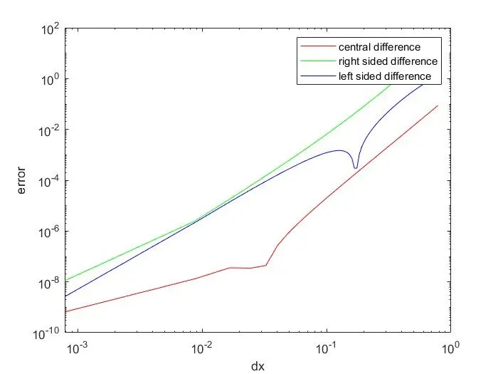
Explaination for code:

1. Writing function code for each schemes seperately

2. Writing matrix A for each taken from taylor table respectively.

3. Calculate analytical derivative

4. Calculate function derivative value in each schemes respectively.

4. Calculate error by taking difference in both values.

5. Merging all schemes in main code by using for loop.

6. Plotting the graph for all 3 schemes, to view the characteristic of each.

Conclusion:

Central difference approximation give least error than right and left sided skewed error.

• Skewed schemes are useful, to calculate the derivative at boundary conditions or end points, where central difference can not be used.