Week 5.1 - Mid term project - Solving the steady and unsteady 2D heat conduction problem
Solving the steady and unsteady 2D heat conduction problem
Aim:
To solve 2D heat convection problem for steady state and transient state analysis.
Objective:
1. To solve Steady state analysis & Transient State Analysis
Given conditions:
Top Boundary = 600 K
Bottom Boundary = 900 K
Left Boundary = 400 K
Right Boundary = 800 K
by using these methods for solving implicit equations.
1. Jacobi
2. Gauss-seidel
3. Successive over-relaxation
Absolute error criteria is 1e-4
2. Write code for both implicit and explicit schemes (Transient Analysis only)
Solution:
Heat equation:
The general 3D equation is termed as:
`((du)/dt)+alpha((d^2T)/dx^2+(d^2T)/dy^2+(d^2T)/dz^2)=0`
First term is time derivative, and second is spacial derivative.
`alpha`is thermal diffusivity.
Steady state heat equation :
The general equation can be reduced to 2D heat eqaution
`(d^2T)/dx^2+(d^2T)/dy^2=0`
Since steady state, time derivative is zero.
By applying second order derivartive the cetral differentiating scheme.
Along x and y direction
`(d^2T)/dx^2=(T_(i-1,j)-2T_(i,j)+T_(i+1,j))/dx^2`
`(d^2T)/dy^2=(T_(i,j-1)-2T_(i,j)+T_(i,j+1))/dy^2`
`T_(i,j)=(1/k)(((T_(i-1,j)+T_(i+1,j))/dx^2)+((T_(i,j-1)+T_(i,j+1))/dy^2)`
where `k=2((dx^2+dy^2)/(dx^2*dy^2))`
considering points,
1.i-1,j=L
2.i,j=P
3.i+1,j=R
4.i,j+1=T
5.i,j-1=B
`T_p=(1/k)((T_L+T_R)/dx^2)+((T_(B)+T_(T))/dy^2)`
Implicit method:
In this method system of eqaution will be obtained and solved.
Iterative solvers are used to compute the unkown, by assigning some guess values and compute error, untill values gets converged where tolerance is given (some higher value).
Iterative solvers methods given as:
1. Jacobi method
2. Guass Siedal method
3. Successive over relaxation(SOR) method
Matlab code:
To solve steady state equation by 3 iterative method,
close all
clear all
clc

%x-axis
nx=10;
%y-axis
ny=10;
%time step
dt=0.0001;
%alpha=a
a=1.5;


T=ones(nx,ny);
%initial cond

for i=1:nx
    %T at top boundary
    T(1,i)=600;
    %T at bottom boundary
    T(ny,i)=900;
end

for j=1:ny
    %T at left boundary
    T(j,1)=400;
    %T at right boundary
   T(j,nx)=800;
end

%Temp at corners
T(1,1)=(T(1,2)+T(2,1))/2;
T(1,nx)=(T(1,nx-1)+T(2,nx))/2;
T(ny,1)=(T(ny-1,1)+T(ny,2))/2;
T(ny,nx)=(T(ny,nx-1)+T(ny-1,nx))/2;

%creating mesh
x=linspace(0,1,nx);
y=linspace(0,1,ny);
dx=x(2)-x(1);
dy=y(2)-y(1);

T_old=T;


itr=1;

%tolerance and error
tol=1e-4;
error=9e9;

%constat
K=((2*(dy^2+dx^2))/(dx^2*dy^2));

%Jacobi method
if itr==1
    itr_n=1;

        %convergence loop

        while(error>tol)
    %space loop
    for i=2:nx-1
        for j=2:ny-1

            T(i,j)=((T_old(i+1,j)+T_old(i-1,j))/(K*dx^2))+((T_old(i,j-1)+T_old(i,j+1))/(K*dy^2));
        end
    end

    error=max(max(abs(T_old-T)));
    T_old=T;
    itr_n=itr_n+1;
        end

    end


%plot graph
figure(1)
colormap=jet;
A=contourf(x,y,T);
clabel(A);
set(gca,'YDir','reverse');
xlabel('x axis');
ylabel('y axis');
title('2D heat conduction Jacobi steady state');
B=sprintf('number of iterations= %d',itr_n);
subtitle(B);


% Guass siedal method

itr=2;

if  itr==2
    itr_n=1;

        while(error>tol)

            for i=2:nx-1;
                for j=2:ny-1;

                    T(i,j)=((T_old(i+1,j)+T(i-1,j))/(K*dx^2))+((T(i,j-1)+T_old(i,j+1))/(K*dy^2));
                end
            end

            error=max(max(abs(T_old-T)));
            T_old=T;
            itr_n=itr_n+1;
        end

    end

figure(2)
colormap=jet;
A=contourf(x,y,T);
clabel(A);
set(gca,'YDir','reverse');
xlabel('x axis');
ylabel('y axis');
title('2D heat conduction Guass Sidel steady state');
B=sprintf('number of iterations= %d',itr_n);
subtitle(B);


%SOR
itr=3;

if itr==3

    itr_n=1;
    %SOR constant
    omega=1.5;

    while(error>tol)

            for i=2:nx-1;
                for j=2:ny-1;

                   T(i,j)= ((1-omega)*(T_old(i,j)))+omega*(((T_old(i+1,j)+T(i-1,j))/(K*dx^2))+((T(i,j-1)+T_old(i,j+1))/(K*dy^2)));
                end
            end

            error=max(max(abs(T_old-T)));
            T_old=T;
            itr_n=itr_n+1;
        end

    end

figure(3)
colormap=jet;
A=contourf(x,y,T);
clabel(A);
set(gca,'YDir','reverse');
xlabel('x axis');
ylabel('y axis');
title('2D heat conduction SOR steady state');
B=sprintf('number of iterations= %d',itr_n);
subtitle(B);
Explaination:
1. Initial conditions are defined: alpha, time steps, axis.
2. Temperature at boundaries and corner points.
3. Tolerance and error are defined, with maximum difference because for higher iterations.
4. Defining constant K.
5. Calculating the Temperature by Jacobi method, for all points of i,j by for loop.
6. Updating the error and T_old.
7. Plotting the graph at different points.
8. Graph is plotted outside the while loop, to obtain end result directly.
9. Similarlly, the process is followed for Guass Siedal and SOR methods.
Graph:
Steady state
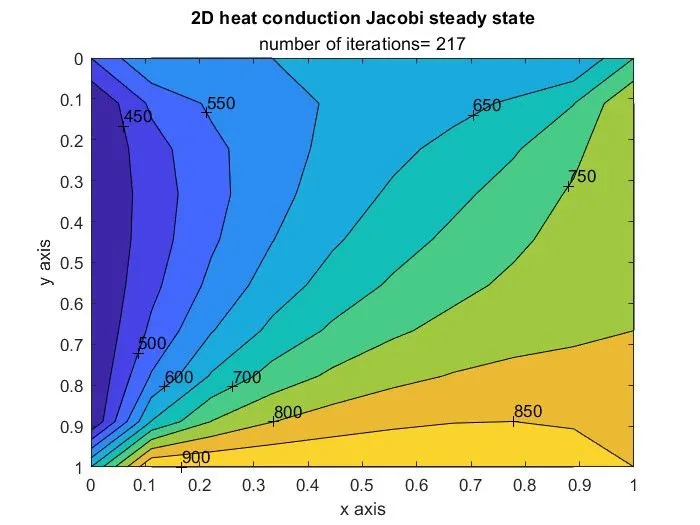
a.Jacobi method:
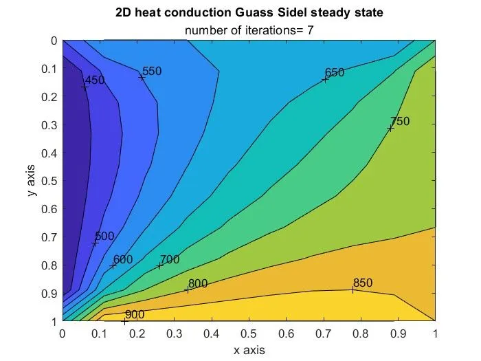
b. Guass Siedal:
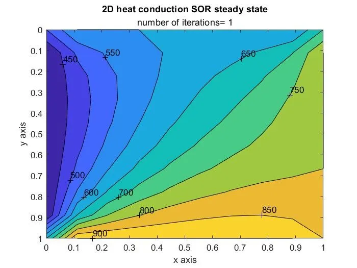
c. SOR method:
Transient analysis:
Explicit method:
In this method equation can be solved by,
`T_p^(n+1)=T_p^n+K1(T_L^n-2T_p^n+T_R^n)+K2(T_T^n-2T_p^n+T_B^n)`
where `K1=alpha*(dt)/dx^2`and `K2=alpha*(dt)/dy^2`
equation ca be solved direclty to compute LHS.
Implicit method:
In this method, it can be solved by
`T_p^(n+1)=T_p^n+K1(T_L^(n+1)-2T_p^(n+1)+T_R^(n+1))+K2(T_T^(n+1)-2T_p^(n+1)+T_B^(n+1))`
where `K1=alpha*(dt)/dx^2`and `K2=alpha*(dt)/dy^2`
Iterative solvers are used to compute the unkown, by assigning some guess values and compute error, untill values gets converged where tolerance is given (some higher value).
Iterative solvers methods given as:
1. Jacobi method
2. Guass Siedal method
3. Successive over relaxation(SOR) method
Matlab code:
To solve using transient analysis method by all 3 implicit method:
close all
clear all
clc

nx=10;
ny=10;
dt=0.001;
%alpha=a
a=1.5;


T=ones(nx,ny);
%initial cond

for i=1:nx
    %T at top boundary
    T(1,i)=600;
    %T at bottom boundary
    T(ny,i)=900;
end

for j=1:ny
    %T at left boundary
    T(j,1)=400;
   T(j,nx)=800;
end

%Temp at corners
T(1,1)=(T(1,2)+T(2,1))/2;
T(1,nx)=(T(1,nx-1)+T(2,nx))/2;
T(ny,1)=(T(ny-1,1)+T(ny,2))/2;
T(ny,nx)=(T(ny,nx-1)+T(ny-1,nx))/2;

%creating mesh
x=linspace(0,1,nx);
y=linspace(0,1,ny);
dx=x(2)-x(1);
dy=y(2)-y(1);

T_old=T;

%CFL or constants
K1=a*(dt/(dx^2));
K2=a*(dt/(dy^2));
CFL=K1+K2;

%defining constants
term1=(1+(2*K1)+(2*K2))^-1;
term2=K1*term1;
term3=K2*term1;

T_prev=T;

%types of solver
itr=1;

%tolerance
tol=1e-4;
nt=1500;
%Jacobi
if itr==1
    %time loop

    for k=1:nt
        error=9e9;

        %convergence loop

        while(error>tol)
    %space loop
    for i=2:nx-1
        for j=2:ny-1


            T(i,j)=(term1*T_prev(i,j))+(term2*(T_old(i+1,j)+T_old(i-1,j)))+(term3*(T_old(i,j-1)+T_old(i,j+1)));
        end
    end

    error=max(abs(T_old-T));
    T_old=T;
    itr=itr+1;
        end
        T_prev=T;
    end


end


%plot graph
figure(1)
colormap=jet;
A=contourf(x,y,T);
clabel(A);
set(gca,'YDir','reverse');
xlabel('x axis');
ylabel('y axis');
title('2D heat conduction Jacobi transient state');
S=sprintf('number of iterations= %d',k);
subtitle(S);


% GS

itr=2;

if  itr==2

    %time loop
    for k=1:nt
        error=9e9;

        while(error>tol)

            for i=2:nx-1;
                for j=2:ny-1;

                    T(i,j)=(term1*T_prev(i,j))+(term2*(T_old(i+1,j)+T(i-1,j)))+(term3*(T_old(i,j-1)+T(i,j+1)));
                end
            end

            error=max(abs(T_old-T));
            T_old=T;
            itr=itr+1;
        end

        T_prev=T;
    end


end
figure(2)
colormap=jet;
A=contourf(x,y,T);
clabel(A);
set(gca,'YDir','reverse');
xlabel('x axis');
ylabel('y axis');
title('2D heat conduction Guass Sidel transient state');
S=sprintf('number of iterations= %d',k);
subtitle(S);


%SOR
itr=3;

if itr==3;
    omega=1.1;
     %time loop
    for k=1:nt
        error=9e9;

        while(error>tol)

            for i=2:nx-1;
                for j=2:ny-1;

                   T(i,j)=(T_old(i,j)*(1-omega))+omega*((term1*T_prev(i,j))+(term2*(T_old(i+1,j)+T(i-1,j)))+(term3*(T_old(i,j-1)+T(i,j+1))));
                end
            end

            error=max(abs(T_old-T));
            T_old=T;
            itr=itr+1;
        end

        T_prev=T;
    end


end
figure(3)
colormap=jet;
A=contourf(x,y,T);
clabel(A);
set(gca,'YDir','reverse');
xlabel('x axis');
ylabel('y axis');
title('2D heat conduction SOR transient state');
S=sprintf('number of iterations= %d',k);
subtitle(S);
Explaination:
1. Initial conditions are defined: alpha, time steps, axis.
2. Temperature at boundaries and corner points.
3. Tolerance and error are defined, with maximum difference because for higher iterations.
4. Defining constant K.
5. Calculating the Temperature by Jacobi method, for all points of i,j by for loop.
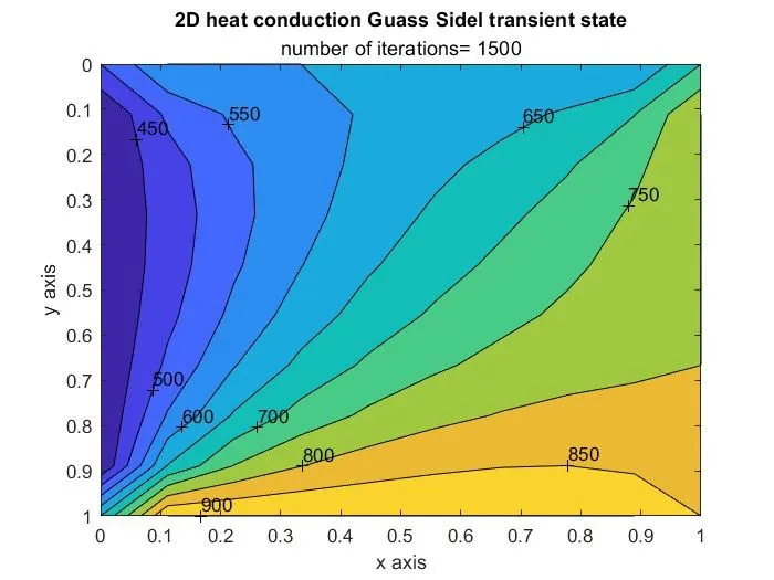
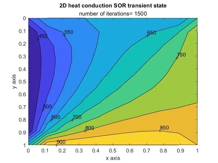
a. nt=1500, 1500 iterations are performed
6. Updating the error and T_old.
7. Plotting the graph at different points.
8. Graph is plotted outside the while loop, to obtain end result directly.
9. Similarlly, the process is followed for Guass Siedal and SOR methods.
Graph :
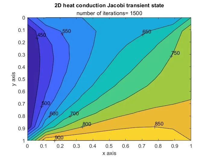
Jacobi method:
Guass siedal:
SOR method:
Matlab code:
To solve transient analysis by expilicit method:
close all
clear all
clc

nx=10;
ny=10;
dt=0.001;
%alpha=a
a=1.5;


T=ones(nx,ny);
%initial cond

for i=1:nx
    %T at top boundary
    T(1,i)=600;
    %T at bottom boundary
    T(ny,i)=900;
end

for j=1:ny
    %T at left boundary
    T(j,1)=400;
   T(j,nx)=800;
end

%Temp at corners
T(1,1)=(T(1,2)+T(2,1))/2;
T(1,nx)=(T(1,nx-1)+T(2,nx))/2;
T(ny,1)=(T(ny-1,1)+T(ny,2))/2;
T(ny,nx)=(T(ny,nx-1)+T(ny-1,nx))/2;

%creating mesh
x=linspace(0,1,nx);
y=linspace(0,1,ny);
dx=x(2)-x(1);
dy=y(2)-y(1);

T_old=T;

%CFL or constants
K1=a*(dt/(dx^2));
K2=a*(dt/(dy^2));
CFL=K1+K2;

%time loop;

nt=1000;

for k=1:nt
    %space loop
    for i=2:nx-1
        for j=2:ny-1

            T(i,j)=(T_old(i,j)+(K1*(T_old(i+1,j)-(2*T_old(i,j))+T_old(i-1,j)))+(K2*(T_old(i,j-1)-2*T_old(i,j)+T_old(i,j+1))));
        end
    end

T_old=T;


end

%plot graph
colormap=jet;
A=contourf(x,y,T);
clabel(A);
set(gca,'YDir','reverse');
xlabel('x axis');
ylabel('y axis');
title('2D heat conduction transient state explicit');
B= sprintf('number of steps= %d, timestep(dt)=%d',k,dt);
subtitle(B);
Explaination:
1. Initial conditions are defined: alpha, time steps, axis.
2. Temperature at boundaries and corner points.
3. Tolerance and error are defined, with maximum difference because for higher iterations.
4. Defining constant K.
5. Calculating the Temperature by explicit method, for all points of i,j by for loop.
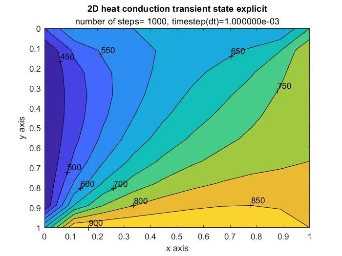
a. assigned nt=1000, for 1000 loop
6. Updating the error and T_old.
7. Plotting the graph at different points.
8. Graph is plotted outside the while loop, to obtain end result directly.
9. Similarlly, the process is followed for Guass Siedal and SOR methods.
Graph:
Conclusion:
The 2D heat equation for steady and transient have been simulated and results obtained is compared.
The number of ierations required in Jacobi method is more than Guass Siedal method than SOR method, to compute the solution.
Jacobi>Guass Siedal>SOR.