Week 8- Moving zones approach in Fluent

1)What are the approaches by which you would model moving zones?

• To model moving zones, two approaches are used,

1. Moving Reference Frame method

A Moving Reference Frame (MRF) is a relatively simple, robust, and efficient steady-state, Computational fluid dynamics modelling technique to simulate rotating machinery. For example, the rotors on a quadcopter can be modelled with MRFs.

The principal reason for employing a moving reference frame is to render a problem which is unsteady in the stationary (inertial) frame steady with respect to the moving frame. For a steadily rotating frame (i.e., the rotational speed is constant), it is possible to transform the equations of fluid motion to the rotating frame such that steady-state solutions are possible.

Another potential use of the MRF model is to compute a flow field that can be used as an initial condition for a transient sliding mesh calculation. This eliminates the need for a startup calculation. The multiple reference frame model should not be used, however, if it is necessary to actually simulate the transients that may occur in rotor-stator solid interactions, the sliding mesh model alone should be used.

there are two types of moving reference frame approaches:

1. Single moving reference frame.
2. Multiple moving reference frame that uses a mixing plane approach.

2. Moving Mesh Approach.

The moving mesh approach is used to model unsteady flows. Generally flows with vortex-induced and for the flows for the interaction of vortex with the bodies, moving mesh approach is used. In moving mesh methods, physical PDEs and a mesh equation derived from equidistribution of an error metrics (so-called the monitor function) are simultaneously solved and meshes are dynamically concentrated on steep regions

2)Which approach would you use to model unsteady phenomena?

Moving Mesh Approach.

3)Simulate rotary motion for the geometry given

• Plot the velocity profile of the fluid motion

setup up the simulation, using the following boundary conditions and cell zone conditions.

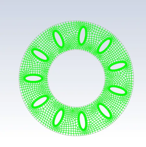
step-1) The meshed model is imported into ansys fluent.

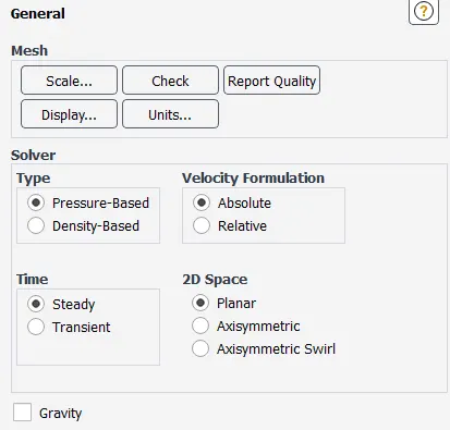
step-2) General settings.

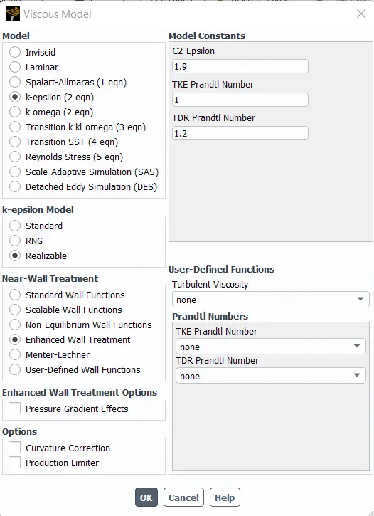
step-3) Viscous Model

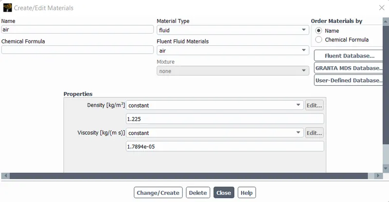
step-4) Selecting material

step-5) Zone motion and material assignment

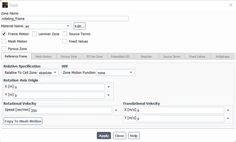
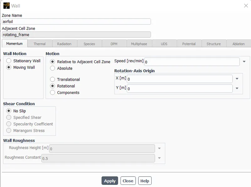
step-6) Boundary Conditions

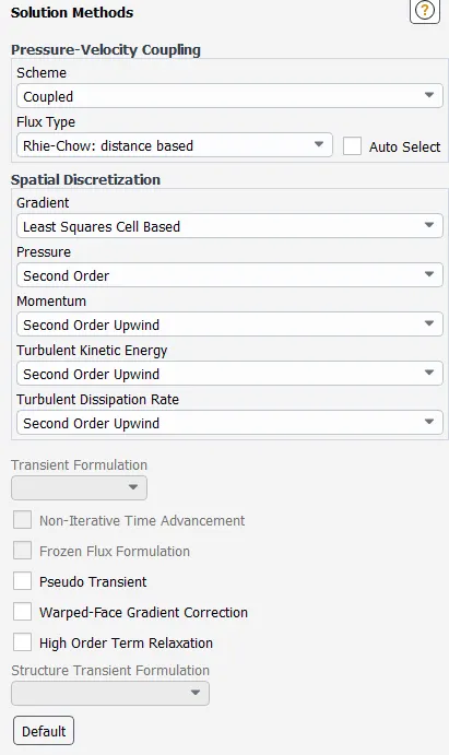
step-7) Solution Methods

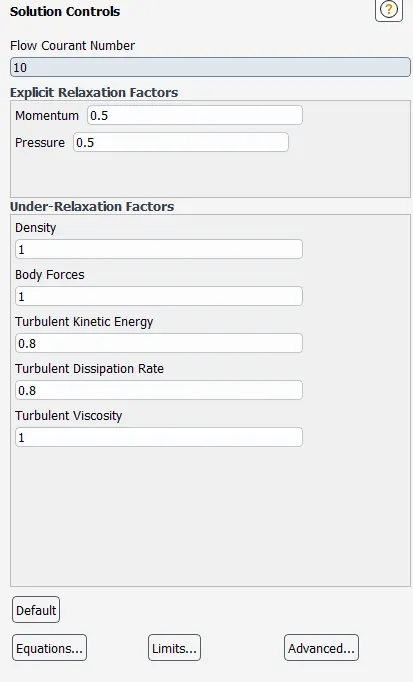
step-8) Solution Controls

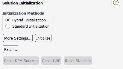
step-9) Initialization Setting

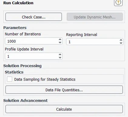
step-10) Running Calculation

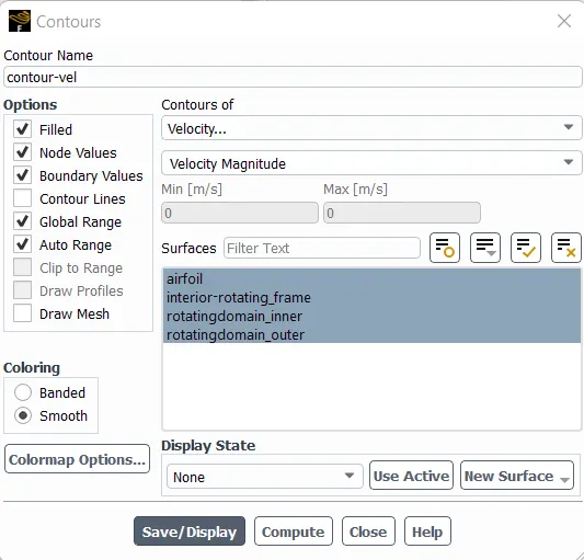
step-11) Velocity contour Plot Settings

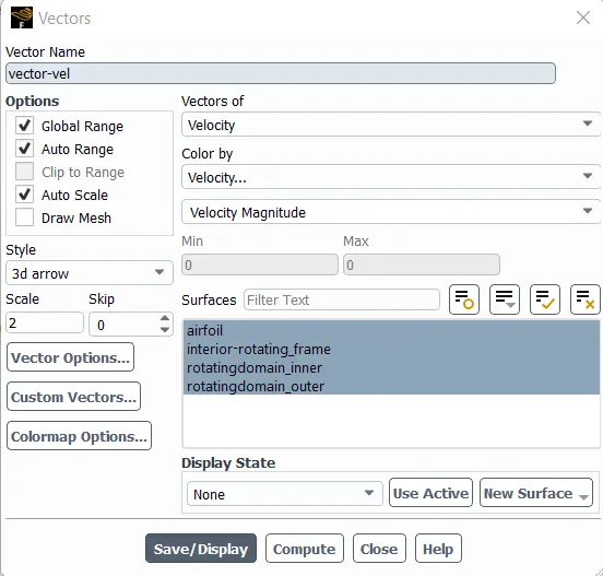
step-12) Velocity Vector Plot Settings

Results

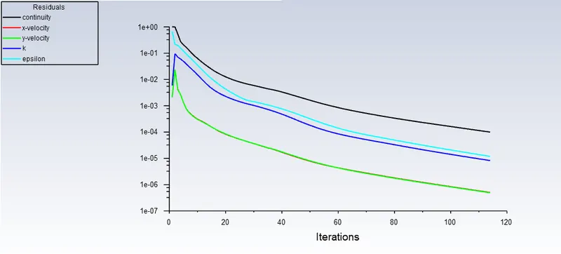
Residuals:

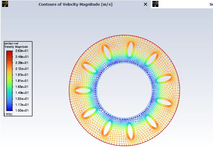
Velocity Contour Plot:

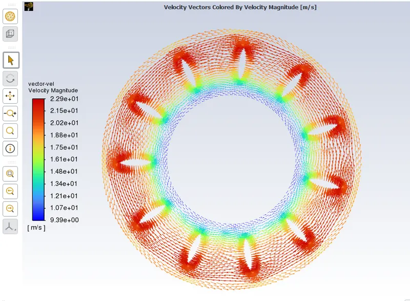
Velocity Vector Plot:

Observation:

From the velocity contours and the velocity vectors, the direction of the flow can be visualized. The velocity is lower in the inner frame, whereas as we move towards the outer frame, the velocity increases.