Simulation of a 1D Super-sonic nozzle flow simulation using Macormack Method

INTRODUCTION:

The following assignment is solved by navier stokes equation in both conservative and non-conservative form

Governing Equations in Non-Conservation Form:

Continuity Equation:

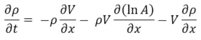
where ρ is the density of the liquid, A is the Area of Cross-Section, V is the Velocity of the liquid, delta t is the time step and x is the Domain Length.

Momentum Equation:

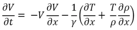
where p.dS is the infinitesimal pressure force. Evaluating it for the entire domain gives us the total pressure force acting at all the points along the domain.

Energy Equation: The energy equation can be changed into the temperature equation by using the ideal gas equation formula.

the energy here expressed is in the form of internal energy associated with the control volume.

MAIN CODE:

clear all
close all
clc

%Inputs 
n=[31,61];
for z=1:length(n)
p=n(z);
x=linspace(0,3,p);
dx=x(2)-x(1);


%Non-Conservative Form
[rho_1,A_1,v_1,T_1,M_1,rho_throat_1,v_throat_1,T_throat_1,M_throat_1,iter_1]=oned_nonconserve(p,x,dx);

%Conservative Form
[rho_2,A_2,v_2,T_2,M_2,rho_throat_2,v_throat_2,T_throat_2,M_throat_2,iter_2]=oned_conservative(p,x,dx);

%Plotting of the Results
% Variation of Parameters with Time Step
figure(z)
subplot(4,1,1)
plot(rho_throat_1,'r');
hold on
plot(rho_throat_2,'b');
ylabel('Density');
title_text_1 =sprintf('Variation of Various Parameters at the Throat with time step (n = %d)',n(z));
title(title_text_1);
legend('Non-Conservative','Conservative','Location','NorthEastOutside');
axis([0 iter_1 0.9*min(rho_throat_1) 1.1*max(rho_throat_1)]);

subplot(4,1,2);
plot(v_throat_1,'r');
hold on
plot(v_throat_2,'b');
ylabel('velocity');
axis([0 iter_1 0.9*min(v_throat_1) 1.1*max(v_throat_1)]);

subplot(4,1,3)
plot(T_throat_1,'r');
hold on
plot(T_throat_2,'b');
ylabel('Temperature');
axis([0 iter_1 0.9*min(T_throat_1) 1.1*max(T_throat_1)]);

subplot(4,1,4)
plot(M_throat_1,'r');
hold on
plot(M_throat_2,'b');
xlabel('No of Iterations');
ylabel('Mach Number');
axis([0 iter_1 0.9*min(M_throat_1) 1.1*max(M_throat_1)]);

% Variation of Mass Flow Rate 
Mass_Flow_Rate_1 = rho_1.*A_1.*v_1;
Mass_Flow_Rate_2 = rho_2.*A_2.*v_2;

figure(z+2)
plot(x,Mass_Flow_Rate_1,'r');
hold on;
plot(x,Mass_Flow_Rate_2,'b');
xlabel('Domain');
ylabel('Normalised Mass Flow Rate');
legend('Non-Conservative','Conservative','Location','North')
title_text_2 = sprintf('Variation of Mass Flow Rate along the Domain (n = %d)',n(z));
title(title_text_2);

% Final Profile of the Various Parameters (Non-Conservative Form)
figure(z+4)
subplot(4,1,1);
plot(x,rho_1);
ylabel('Density');
title_text_3 = sprintf('Final Profile of the Various Parameters (Non-Conservative Form) along the Domain (n = %d)n Number of Iterations = %d',n(z),iter_1);
title(title_text_3);
axis([0 3 0.9*min(rho_1) 1.1*max(rho_1)]);

subplot(4,1,2);
plot(x,T_1);
ylabel('Temperature');
axis([0 3 0.9*min(T_1) 1.1*max(T_1)]);


subplot(4,1,3);
plot(x,v_1);
ylabel('Velocity');
axis([0 3 0.9*min(v_1) 1.1*max(v_1)]);

subplot(4,1,4);
plot(M_1);
xlabel('Length of Domain (m)');
ylabel('Mach Number');
axis([0 3 0.9*min(M_1) 1.1*max(M_1)]);

% Final Profile of the Various Parameters (Conservative Form)
figure(z+6)
subplot(4,1,1);
plot(x,rho_2);
ylabel('Density');
title_text_3 = sprintf('Final Profile of the Various Parameters (Conservative Form) along the Domain (n = %d)n Number of Iterations = %d',n(z),iter_2);
title(title_text_3);
axis([0 3 0.9*min(rho_2) 1.1*max(rho_2)]);

subplot(4,1,2);
plot(x,T_2);
ylabel('Temperature');
axis([0 3 0.9*min(T_2) 1.1*max(T_2)]);


subplot(4,1,3);
plot(x,v_2);
ylabel('Velocity');
axis([0 3 0.9*min(v_2) 1.1*max(v_2)]);

subplot(4,1,4);
plot(M_2);
xlabel('Length of Domain (m)');
ylabel('Mach Number');
axis([0 3 0.9*min(M_2) 1.1*max(M_2)]);

end

The MacCormack method is a weighted average method that uses both the forward as well as backward differencing schemes to solve the discretized equations.

Solving the Non-Conservative Form with MacCormack Method

After obtaining the Non-Conservative form of the Continuity, Momentum and the Energy equation, the following set of instructions are followed:

1.Nozzle Shape and Initial Conditions: The area of the Nozzle is a function of the domain vector x and is given by the equation:

The primitive variables have their intial profiles given by:

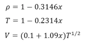
2.The Finite Difference Equations: The above partial differential equations have been discretized by both the Forward as well as Backward Differencing Schemes. The discretization takes place in two steps; first is the Predictor Step which involves discretizing them using the forward differencing scheme and then using the Corrector Step which uses the backward differencing schemes for the discretization.

Predictor Step:

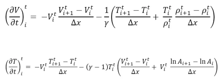
The values obtained in the predictor step will now be used to calculate the values of the primitive variables for the next time step as follows:

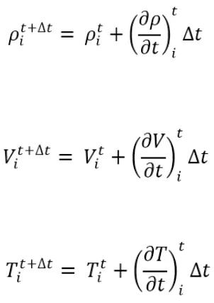
The values of the primitive variables obtained in the predictor step will now be used for the corrector step.

Corrector Step:

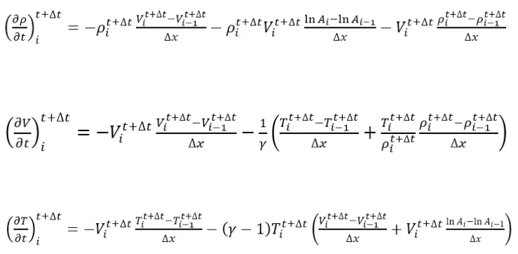
Calculation of the average of the predictor and the corrector step:

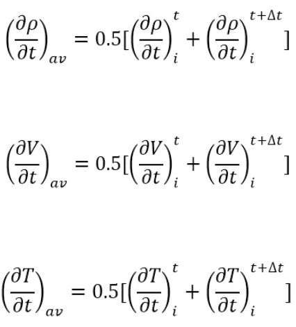
The final values of the primitive variables are calculated by the equation:

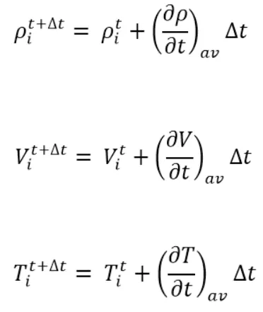
3. Calculation of Time Step: The calculation of the time step is followed by the equation given as:

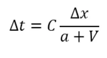
since a and V are the vectors generating an array of values hence the time step is the minimum of the above formula. Here C is the Courant Number which is also the criteria of the convergence for the solution.

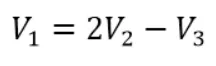
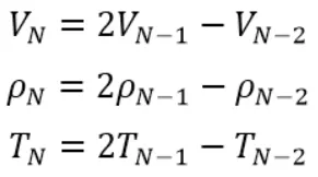
4. Boundary Conditions: The boundary conditions will be given at both the inlet and the outlet of the domain.

Inflow Boundary Condition:

Outflow Boudary Condition:

CODE FOR NON-CONSERVTIVE FORM:

function [rho_1,A_1,v_1,T_1,M_1,rho_throat_1,v_throat_1,T_throat_1,M_throat_1,iter_1] =oned_nonconserve(p,x,dx)

% Initial profiles
rho_1=1-0.3146*x;
T_1 = 1-0.2314*x;
v_1=(0.1+1.09*x).*T_1.^0.5;
M_1=zeros(1,p-1);
A_1=1+2.2*(x-1.5).^2;
gamma=1.4;

% Calculation of Time Step
C=0.5;
a=T_1.^0.5;
dt=min(C*(dx)./(a+v_1));
error=1e5;
tol=1e-6;

% Copy of the Initial Values
rho_old=rho_1;
T_old=T_1;
v_old=v_1;
iter_1=0;

% Predictor Terms
drhodt_p=zeros(1,p-1);
dvdt_p=zeros(1,p-1);
dTdt_p=zeros(1,p-1);

% Correctoer Terms
drhodt_c=zeros(1,p-1);
dvdt_c=zeros(1,p-1);
dTdt_c=zeros(1,p-1);

%Outer Time Loop 
while error>tol
iter_1=iter_1+1;

% Predictor Step 
for j=2:p-1
dvdx=(v_1(j+1)-v_1(j))/dx;
drhodx=(rho_1(j+1)-rho_1(j))/dx;
dTdx=(T_1(j+1)-T_1(j))/dx;
dlogadx=(log(A_1(j+1))-log(A_1(j)))/dx;

% Continuity Equation
drhodt_p(j)=-rho_1(j)*dvdx-rho_1(j)*v_1(j)*dlogadx-v_1(j)*drhodx;

% Momentum Equation
dvdt_p(j)=-v_1(j)*dvdx-(1/gamma)*(dTdx+(T_1(j)/rho_1(j))*drhodx);

% Temperature Equation
dTdt_p(j)=-v_1(j)*dTdx-(gamma-1)*T_1(j)*(dvdx+v_1(j)*dlogadx);

% Predictor Update
rho_1(j)=rho_1(j)+drhodt_p(j)*dt;
v_1(j)=v_1(j)+dvdt_p(j)*dt;
T_1(j)=T_1(j)+dTdt_p(j)*dt;
end

% Corrector Step
for j=2:p-1
dvdx = (v_1(j) - v_1(j-1))/dx;
drhodx=(rho_1(j)-rho_1(j-1))/dx;
dTdx=(T_1(j)-T_1(j-1))/dx;
dlogadx=(log(A_1(j))-log(A_1(j-1)))/dx;

% Continuity Equation
drhodt_c(j)=-rho_1(j)*dvdx-rho_1(j)*v_1(j)*dlogadx-v_1(j)*drhodx; 

 % Momentum Equation
dvdt_c(j)=-v_1(j)*dvdx-(1/gamma)*(dTdx+(T_1(j)/rho_1(j))*drhodx);

% Temperature Equation
dTdt_c(j)=-v_1(j)*dTdx-(gamma-1)*T_1(j)*(dvdx+v_1(j)*dlogadx);
end

% Average of predictor and Corrector steps
drhodt=0.5*(drhodt_p+drhodt_c);
dvdt=0.5*(dvdt_p+dvdt_c);
dTdt=0.5*(dTdt_p+dTdt_c);


% Final Solution Update
for i=2:p-1
rho_1(i)=rho_old(i)+drhodt(i)*dt;
v_1(i)=v_old(i)+dvdt(i)*dt;
T_1(i)=T_old(i)+dTdt(i)*dt;
M_1(i)=v_1(i).*T_1(i).^0.5;
end

% Variation of the Parameters at the throat with time Step
rho_throat_1(iter_1)=rho_1(1,(p-1)/2);
v_throat_1(iter_1)=v_1(1,(p-1)/2);
T_throat_1(iter_1)=T_1(1,(p-1)/2);
M_throat_1(iter_1)=M_1(1,(p-1)/2);

% Applying Boundary Conditions

% Inlet
v_1(1)=2*v_1(2)-v_1(3);

% Outlet
v_1(p)=2*v_1(p-1)-v_1(p-2);
rho_1(p)=2*rho_1(p-1)-rho_1(p-2);
T_1(p)=2*T_1(p-1)-T_1(p-2);


% Updating the old values
error=max(abs(rho_old-rho_1));
rho_old=rho_1;
T_old=T_1;
v_old=v_1;
end

end

Solving the Conservative Form with the MacCormack Method

1.The Basic Equations in Conservation Form:

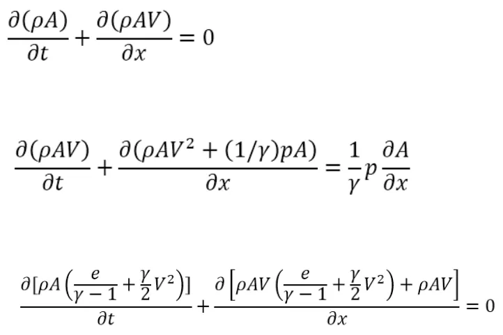
2. Conversion of the above equations : The above equations are very complex in nature and hence solving them directly is a very tedious task. Hence to overcome this problem the primary variables are expressed in terms of the solution variables and the flux variables as follows:

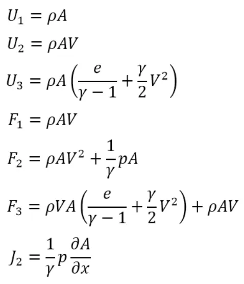
where U is the solution vector, F is the Flux Vector and J is the source term. Now the above Conservation Equations become:

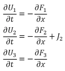
3. Expressing the Flux and Source Terms in the Form of Solution Vectors: By solving for these U1, U2 and U3 we can substitute the value and find the value of the primitive variables. Now the next step is to express the flux variables in the form of solution variables.

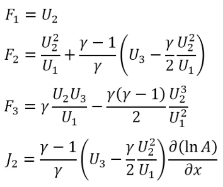
4. Solving the Soluton vector equations with the Standard MacCormack Procedure: Now that we have to solve for the Solution Variables, we can now proceed with the solution as we did for solving the Non-Conservative Equations.
5. Boundary Conditons: The boundary conditions will be applied both at the inlet and the outlet as we did in the previous case.

Inflow Boundary Conditions:

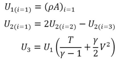
Outflow Boundary Conditions:

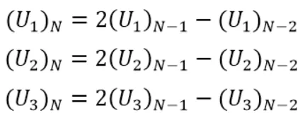
6. Initial Conditions: The initial conditions are provided in terms of the primitive variables as follows:

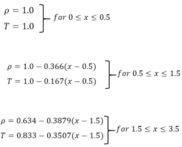
7. Calculation of Time Step: The time step here has been calculated with the same formaula as used in the Non-Conservation form.

CODE FOR CONSERVATIVE FORM:

function [rho_2,A_2,v_2,T_2,M_2,rho_throat_2,v_throat_2,T_throat_2,M_throat_2,iter_2] =oned_conservative(p,x,dx)

% Initial profiles of Primirtive Variables

% Pre Allocation of Prmtive Variables
rho_2=zeros(1,p);
T_2=zeros(1,p);

for i=1:p
if (x(i)>=0)&&(x(i)<0.5)
rho_2(i)=1.0;
T_2(i)=1.0;

elseif (x(i)>=0.5)&&(x(i)<1.5)
rho_2(i)=1.0-0.366*(x(i)-0.5);
T_2(i)=1.0-0.167*(x(i)-0.5);

else
rho_2(i)=0.634-0.3879*(x(i)-1.5);
T_2(i)=0.833-0.3507*(x(i)-1.5);
end
end

A_2=1+2.2.*(x-1.5).^2;
v_2=0.59./(rho_2.*A_2);
e_2=T_2;
gamma=1.4;

% Initial profiles of Dependant Variables

% Solution Vectors
U1=rho_2.*A_2;
U2=U1.*v_2;
U3=rho_2.*((e_2/(gamma-1))+(gamma/2).*v_2.^2).*A_2;

% Flux Vectors
F1=U2;
F2=((U2.^2)./U1)+((gamma-1)/gamma)*(U3-(gamma/2)*((U2.^2)./U1));
F3=gamma*((U2.*U3)./U1)-(gamma*(gamma-1))/2*((U2.^3)./(U1.^2));

% Pre-Allocation of Variables
J2=zeros(1,p-1);

dU1dt_p=zeros(1,p-1);
dU2dt_p=zeros(1,p-1);
dU3dt_p=zeros(1,p-1);

dU1dt_c=zeros(1,p-1);
dU2dt_c=zeros(1,p-1);
dU3dt_c=zeros(1,p-1);

% Source Term
for i=1:p-1
J2(i)=(1/gamma)*(rho_2(i))*(T_2(i))*(A_2(i+1)-A_2(i))/dx;
end

% Simulation Parameters
C=0.5;
error=1e6;
tol=1e-6;
iter_2=0;
rho_old=rho_2;


% Computational Loop
while error>tol

% Calculation of Time Step
a=T_2.^0.5;
dt=min((C*dx)./(a + v_2));

% Updating the Initial Variables
U1_old=U1;
U2_old=U2;
U3_old=U3;

% Updating Iterations
iter_2=iter_2+1;

% Predictor Step
for j=2:p-1

% Flux Vectors    
F1(j)=U2(j);
F2(j)=((U2(j)^2)/U1(j))+((gamma-1)/gamma)*(U3(j)-((gamma/2)*((U2(j)^2)/U1(j))));
F3(j)=gamma*((U2(j)*U3(j))/U1(j))-(0.5*gamma*(gamma-1))*((U2(j)^3)/(U1(j)^2));

% Source Vector
J2(j)=(1/gamma)*(rho_2(j))*(T_2(j))*((A_2(j+1)-A_2(j))/dx);

% Discritization Terms
dF1dx=(F1(j+1)-F1(j))/dx;
dF2dx=(F2(j+1)-F2(j))/dx;
dF3dx=(F3(j+1)-F3(j))/dx;  

% Conitinuity Equation
dU1dt_p(j)=-dF1dx;

% Momentum Equation
dU2dt_p(j)=-dF2dx+J2(j);

% Energy Equation
dU3dt_p(j)=-dF3dx;

% Solution Vector Update
U1(j)=U1(j)+dU1dt_p(j)*dt;
U2(j)=U2(j)+dU2dt_p(j)*dt;
U3(j)=U3(j)+dU3dt_p(j)*dt;

% Primitive Values
rho_2(j)=U1(j)/A_2(j);
v_2(j)=U2(j)/U1(j);
T_2(j)=(gamma-1)*((U3(j)/U1(j))-(gamma/2)*((U2(j)/U1(j))^2));

end

% Flux Vectors
F1=U2;
F2=(U2.^2./U1)+((gamma-1)/gamma)*((U3-((gamma/2)*((U2.^2)./U1))));
F3=((gamma*U2.*U3)./U1)-((gamma*(gamma-1)*0.5*(U2.^3))./(U1.^2));

% Corrector Step
for j=2:p-1

% Source Term
J2=(1/gamma)*(rho_2(j)).*(T_2(j)).*((A_2(j)-A_2(j-1))/dx);

% Discritization Terms
dF1dx=(F1(j)-F1(j-1))/dx;
dF2dx=(F2(j)-F2(j-1))/dx;
dF3dx=(F3(j)-F3(j-1))/dx;

% Conitinuity Equation
dU1dt_c(j)=-dF1dx;

% Momentum Equation
dU2dt_c(j)=-dF2dx+J2;

% Energy Equation
dU3dt_c(j)=-dF3dx;  

end

% Average of Predictor and Corrector
dU1dt = 0.5*(dU1dt_p + dU1dt_c);
dU2dt = 0.5*(dU2dt_p + dU2dt_c);
dU3dt = 0.5*(dU3dt_p + dU3dt_c);

% Final Solution Update
for i=2:p-1
U1(i)=U1_old(i)+dU1dt(i)*dt;
U2(i)=U2_old(i)+dU2dt(i)*dt;
U3(i)=U3_old(i)+dU3dt(i)*dt;
end

% Final Values of the Primitves
rho_2=U1./A_2;
v_2=U2./U1;
T_2=(gamma-1)*((U3./U1)-(gamma/2)*v_2.^2);
m=rho_2.*A_2.*v_2;
M_2=v_2./(T_2.^0.5);

% Variation of the Parameters at the throat with time Step
rho_throat_2(iter_2)=rho_2(1,(p-1)/2);
v_throat_2(iter_2)=v_2(1,(p-1)/2);
T_throat_2(iter_2)=T_2(1,(p-1)/2);
M_throat_2(iter_2)=M_2(1,(p-1)/2);

% Applying Boundary Conditions

% Inlet Boundary Conditions
U1(1)=rho_2(1)*A_2(1);
U2(1)=2*U2(2)-U2(3);
U3(1)=U1(1)*(T_2(1)/(gamma-1)+(gamma/2)*v_2(1)^2);

% Outlet Boundary Conditions
U1(p)=2*U1(p-1)-U1(p-2);
U2(p)=2*U2(p-1)-U2(p-2);
U3(p)=2*U3(p-1)-U3(p-2);

% Updating the old values
error=max(abs(rho_old-rho_2));
rho_old=rho_2;
end
end

RESULTS:

1)Grid Dependance Test:

The results of CFD analysis largely depends upon the spacing between the adjacent grid points in the domain we have provided. Grid Independance means that the solution or the result of our analysis should be unaffected from the change in the grid points. To analyse this effect we initially choose 31 grid points and then solved for the same unknowns with 61 grid points. And then analysed the result.

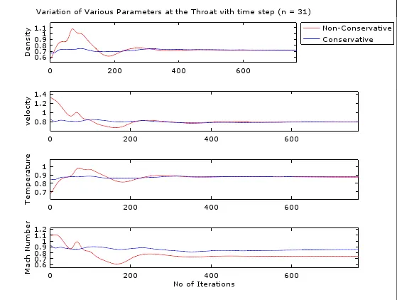
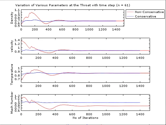
PLOT OF TIME WISE VARIATION OF PRESSURE, TEMPERATURE, VELOCITY AND MACH NUMBER AT n=31,61

AT n=31

AT n=61

OBSERVATION:

AT n=31: we canc see in the plot that the stability is achieved by the non-conservative form earlier than the conservative form but the amplitude of the initial variations is also higher in the non-conservation form (the convergence criteria has been kept equal for both the cases).

AT n=61 :As we can see in the plot that there is a slight variation in the profile with 61 grid points of the various parameters as compared to the variation for 31 grid points hence we can conclude that our solution is not grid independent.

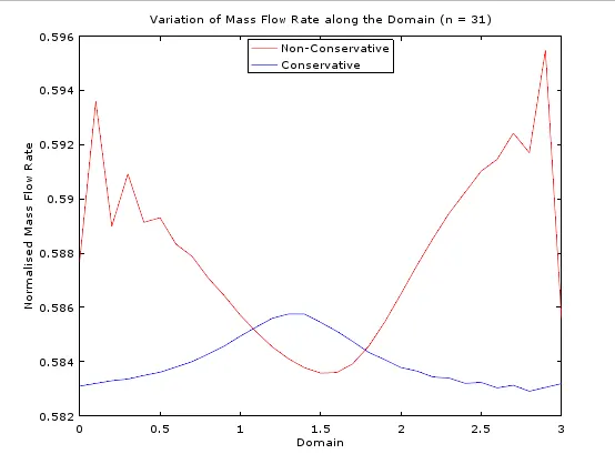
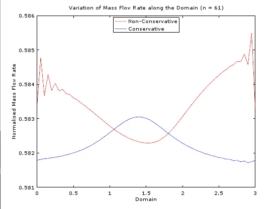
2) MASS FLOW RATE (AT n=31,61)

AT n=31

AT n=61

OBSERVATION:

In the plot we can see that the profile of the conservative form is much closer to the exact solution and on the other hand the variation in the mass flow rate of the non-conservative form is larger and also far from the exact analytical solution.The conclusion made for the comparison of the Mass Flow Rate for 31 grid points hold good even for the 61 grid points as there may only be a slight variation in profiles.

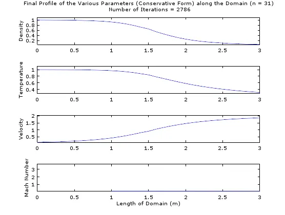
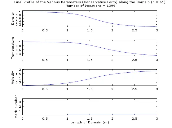
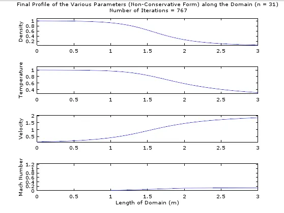
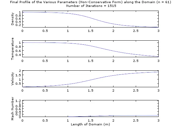
3) FINAL PROFILE OF VARIOUS PARAMETERS IN CONSERVATIVE AND NON-CONSERVATIVE FROM (AT n=31,61)

CONSERVATIVE FORM

AT n=31

AT n=61

NON-CONSERVATIVE FORM

AT n=31

AT n=61

OBSERVATION:

1.In the plots we can see that the profile of the parametrs is similar to that of the the exact analytical solution.

2.The above plots show the minimum number of iterations required in each case in order to reach the desired convergence criteria. The following table contains the data for the minimum number of cycles required to reach the desired error criteria:

We can not clearly conclude that which form of equation can lead to faster convergence because it depends upon various factors and out of those factors saw the effect grid dependance. Hence claiming one of the method to be faster than the other is out of scope of this project.