Mid term project - Solving the steady and unsteady 2D heat conduction problem
We make the assumptions as there is no convection, no internal heat generation and no change of temperature gradient with respect to time, therefore the generalised energy equation in 2D becomes as:
∂2T∂x2+∂2T∂y2=0
∂2T∂x2+∂2T∂y2=0
1. Steady State Solution
Solving the steady state equations does not involve time marching therefore the temperature gradient do not change with respect to time.
We discritize spatial term by central differencing:
∂2T∂x2=Ti−1,j−2Ti,j+Ti+1,jΔx2
∂2T∂x2=Ti-1,j-2Ti,j+Ti+1,jΔx2
∂2T∂y2=Ti,j−1−2Ti,j+Ti,j+1Δy2
∂2T∂y2=Ti,j-1-2Ti,j+Ti,j+1Δy2
therefore we get
Ti−1,j−2Ti,j+Ti+1,jΔx2+Ti,j−1−2Ti,j+Ti,j+1Δy2=0
Ti-1,j-2Ti,j+Ti+1,jΔx2+Ti,j-1-2Ti,j+Ti,j+1Δy2=0
we take
Δx=ΔyΔx=Δy
Ti=14(Ti−1,j+Ti+1,j+Ti,j−1+Ti,j+1)
Ti=14(Ti-1,j+Ti+1,j+Ti,j-1+Ti,j+1)
Following are the codes for steady state analysis:
%Steady State Solution
clear all
close all
clc
%Step 1:
%First lets Initial the given condition

L = 1;
nx = 20;
ny = 20;
x = linspace(0,L,nx);
y = linspace(0,L,ny);
dx = x(2)-x(1);
dy = y(2)-y(1);
error = 9e9;
tol = 1e-4;


% Step 2:
% Define boundary condition

T_L = 400;
T_T = 600;
T_R = 800;
T_B = 900;
T = ones(nx,ny);

% Temperature at Boundary
T(2:ny-1,1) = T_L;
T(2:ny-1,nx) = T_R;
T(1,2:nx-1) = T_T;
T(nx,2:ny-1) = T_B;

% Temperature at the corner by  average value temperature
T(1,1) = (T_T + T_L)/2;
T(nx,ny) = (T_R + T_B)/2;
T(1,ny) = (T_T + T_R)/2;
T(nx,1) = (T_L + T_B)/2;

k1 = (dx^2)/(2*(dx^2+dy^2));
k2 = (dy^2)/(2*(dx^2+dy^2));
i_s=1;  %Selection of method

if i_s==1;
jacobi_iter(T,x,y,nx,ny,tol,error,k1,k2);

elseif i_s==2;
gauss_iter(T,x,y,nx,ny,tol,error,k1,k2);

elseif i_s==3;
sor_iter(T,x,y,nx,ny,tol,error,k1,k2);

end
%Jacobi Iteration
function  jacobi_iter(T,x,y,nx,ny,tol,error,k1,k2)


[X, Y] = meshgrid(x,y);
Told = T;
tic

jacobi_iterr = 1;
while(error>tol)
for i = 2:nx-1
for j = 2:ny-1
T(i,j)=k1*(Told(i-1,j)+Told(i+1,j))+k2*(Told(i,j-1)+Told(i,j+1))
end
end


error = max(max(abs(Told-T)));
Told = T;
jacobi_iterr = jacobi_iterr+1;

end


time_taken=toc;
figure(1)
contourf(x,y,T);
[a b] = contourf(x,y,T);
clabel(a,b);
xlabel('X')
ylabel('Y')
colorbar

title_text = sprintf('Jacobi No of iteration = %d' , jacobi_iterr);
title(title_text)
file_text = sprintf('Jacobi.png');
saveas(gca,file_text);
fprintf('Number of iterations done are %d n',jacobi_iterr);
fprintf('Time taken for solving equation is %f n',time_taken);

end
%Gauss Iteration
function gauss_iter(T,x,y,nx,ny,tol,error,k1,k2)
[X, Y] = meshgrid(x,y);
Told = T;
tic
gs_iter = 1;
while(error>tol)
for i = 2:nx-1
for j = 2:ny-1
T(i,j) = k1*(T(i,j-1)+Told(i,j+1))+k2*(T(i-1,j)+Told(i+1,j));
end
end
error =max(max(abs(Told-T)));
Told = T;
gs_iter = gs_iter+1;
end
time_taken=toc;
figure(1)
contourf(x,y,T);
[a b] = contourf(x,y,T);
clabel(a,b);
colorbar
title_text = sprintf('Gauss no of iteration = %d' , gs_iter);
title(title_text)
file_text = sprintf('G_S.png');
saveas(gca,file_text);
fprintf('Number of iterations done are %d n',gs_iter);
fprintf('Time taken for solving equation is %f n',time_taken);
end%SOR Iteration
function sor_iter(T,x,y,nx,ny,tol,error,k1,k2)
% relaxation factor calculation
z=cos(pi/nx)+cos(pi/ny);
omega = 4/(2+sqrt(4-z^2));
Told = T;
[X Y] = meshgrid(x,y);
sor_iter = 1;
while(error>tol)
for i = 2:nx-1
for j = 2:ny-1
T(i,j) = omega*(k1*(T(i,j-1)+T(i,j+1))+k2*(T(i-1,j)+T(i+1,j)))+(1-omega)*Told(i,j);
end
end
error = max(max(abs(Told-T)));
Told = T;
sor_iter = sor_iter+1;
end
time_taken=toc;
figure(1)
contourf(x,y,T);
[a b] = contourf(x,y,T);
clabel(a,b);
colorbar;
title_text = sprintf('Sor no of iteration = %d' , sor_iter);
title(title_text)
file_text = sprintf('S-SOR.png');
saveas(gca,file_text);
fprintf('Relaxation factor considered is %d n',omega);
fprintf('Number of iterations done are %d n',sor_iter);
fprintf('Time taken for solving equation is %f n',time_taken);
endOutput:
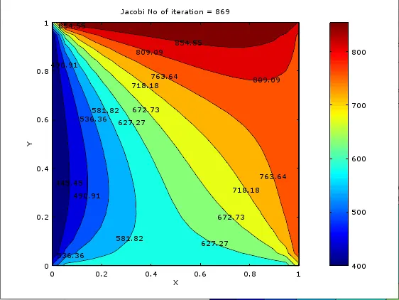
1.Jacobi Method:
 >>>>
>>>>
Number of iterations done are 869
Time taken for solving equation is 361.586736
2.Gauss Seidel Method:
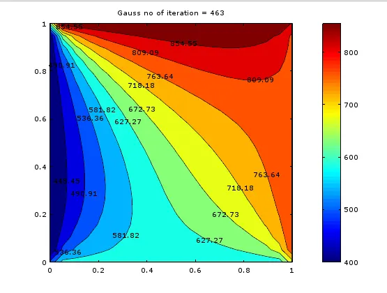
Number of iterations done are 463
Time taken for solving equation is 0.005830
3.Successive Over Relaxation Method:
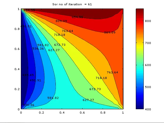
Relaxation factor considered is 1.729454e+00
Number of iterations done are 61
Time taken for solving equation is 0.002747
observation:
From the above results we can deduce that amongst the three iterative methods we get the results faster and with less error in the case of Successive Over Relaxation method than the Gauss Seidel method which is faster than the Jacobi method .
2.Unsteady State Solution:
The Generalised energy equation in 2D becomes as :
∂2T∂x2+∂2T∂y2=α∂T∂t
∂2T∂x2+∂2T∂y2=α∂T∂t
the above equation is obtained by making assumptions that there is no convection , no internal heat generation or dessipation and aplha being constant .
We discritize spatial term by central differencing:
∂2T∂x2=Ti−1,j−2Ti,j+Ti+1,jΔx2
∂2T∂x2=Ti-1,j-2Ti,j+Ti+1,jΔx2
∂2T∂y2=Ti,j−1−2Ti,j+Ti,j+1Δy2
∂2T∂y2=Ti,j-1-2Ti,j+Ti,j+1Δy2
we discritize temporal terms by Forward differencing:
∂T∂t=(Tn+1)i,j−(Tn)i,jΔt
∂T∂t=(Tn+1)i,j-(Tn)i,jΔt
hence ,
(Ti−1,j−2Ti,j+Ti+1,j)n+1Δx2+(Ti,j−1−2Ti,j+Ti,j+1)n+1Δy2=(Tn+1)i,j−(Tn)i,jΔt
(Ti-1,j-2Ti,j+Ti+1,j)n+1Δx2+(Ti,j-1-2Ti,j+Ti,j+1)n+1Δy2=(Tn+1)i,j-(Tn)i,jΔt
we have defined 2 constants namely k4 and k5
K4=αΔt(Δx)2
K4=αΔt(Δx)2
K5=αΔt(Δy)2
K5=αΔt(Δy)2
as
Δx=Δy
hence:
(Tn+1)i,j=(Tn)i,j+K4((Tn+1)i−1,j−2(Tn+1)i,j+(Tn+1)i+1,j)+K5((Tn+1)i,j−1−2(Tn+1)i,j+(Tn+1)i,j+1)
(Tn+1)i,j=(Tn)i,j+K4((Tn+1)i-1,j-2(Tn+1)i,j+(Tn+1)i+1,j)+K5((Tn+1)i,j-1-2(Tn+1)i,j+(Tn+1)i,j+1)
therefore:
(Tn+1)i,j=(Tn)i,j+(K4(Ti−1,j+Ti+1,j)+K5(Ti,j−1+Ti,j+1))n+11+2K4+2K5
(Tn+1)i,j=(Tn)i,j+(K4(Ti-1,j+Ti+1,j)+K5(Ti,j-1+Ti,j+1))n+11+2K4+2K5
In Transient condition Temperature changes with time and reaches a steady state. The above equation is iterated both explicitly and implicitly.
2.1 EXPLICIT METHOD:
In explicit method the temperature at next level is calculated by means of surrounding temperature values and increasing the time steps i.e dt shall result in oscillation of result and the solution diverges from the original result.
Following is the code for 2-D Transient Unsteady equation solved explicitly:
%  2D Transient State Heat Conduction Equation explicitly:
clear all
close all
clc

%Step 1:

%First lets Initial the given condition

L=1;
nx= 20;
ny = 20;
x=linspace(0,L,nx);
y=linspace(0,L,ny);
dx=x(2)-x(1);
dy= y(2)-y(1);
dt = 30;
nt = 1000;
tol = 1e-4;
error = 9e9;

% Step 2:

% Define boundary condition

T_L = 400;
T_T = 600;
T_R = 800;
T_B = 900;
T =ones(nx,ny);

% Temperature at Boundary
T(2:ny-1,1) = T_L;
T(2:ny-1,nx) = T_R;
T(1,2:nx-1) = T_T;
T(nx,2:ny-1) = T_B;

% Temperature at corner (average temperature)
T(1,1) = (T_T + T_L)/2;
T(nx,ny) = (T_R + T_B)/2;
T(1,ny) = (T_T + T_R)/2;
T(nx,1) = (T_L + T_B)/2;

alpha=2.3e-5;
CFL = alpha*dt/(dx^2);


k4 = (alpha*dt)/(dx^2);
k5 = (alpha*dt)/(dy^2);
[X,Y] = meshgrid(x,y);
Told = T;
T_prev_dt = Told;
tic;
counter = 0;
for k = 1:nt

% Jacobi explicit Iteration Scheme
for i = 2:nx-1
for j = 2:ny-1
term1 = Told(i,j);
term2 = k4*(Told(i-1,j)-2*Told(i,j)+Told(i+1,j));
term3 = k5*(Told(i,j-1)-2*Told(i,j)+Told(i,j+1));
T(i,j) = term1+term2+term3;
end
end
Told = T;
counter = counter+1;
end
time_required = toc;
figure(1)
[a,b] = contourf(X,Y,T);
colorbar;
clabel(a,b);
title(sprintf('2D Unsteady state heat conduction-- Explicit Method n Number of iterations: %d',counter));
xlabel('X');
ylabel('Y');
hold on
saveas(gca,'2D Unsteady state heat conduction -Explicit Method .png');
fprintf('Number of iterations done are %d n',counter);
fprintf('Time taken for solving equation is %f n',time_required);
fprintf('cfl number %f',CFL)
Graph 2D Unsteady Transient Heat conduction by Explicit Method:
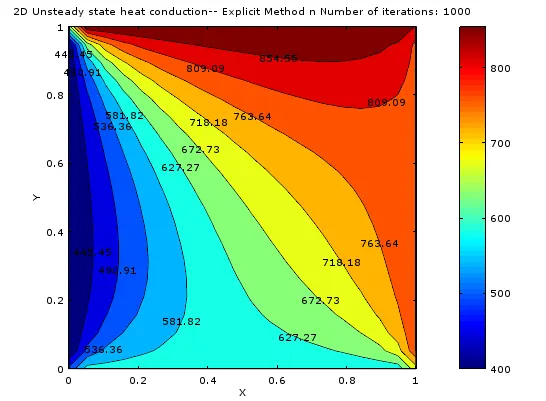
Number of iterations done are 1000
Time taken for solving equation is 0.017363
cfl number 0.249090
conclusion:
The above plot shows the distribution of the temperature field. It can be clearly inferred that based upon boundary conditions the distribution of temperature starts from the edges and goes to the centre and as a result the temperature is minimum around the centre.
2.2 IMPLICIT METHOD:
Following is the code for 2 D Transient Unsteady equation solved Implicitly:
%  TwoD_Unsteady_Transient_state_Heat_Conduction_Equation_implicitly:
clear all
close all
clc
%Step 1:
%First lets Initial the given condition

L=1;
nx= 20;
ny =20;
x=linspace(0,L,nx);
y=linspace(0,L,ny);
dx=x(2)-x(1);
dy= y(2)-y(1);
dt = 30;
nt = 1000;
tol = 1e-4;
error = 9e9;

% Step 2:
% Define boundary condition

T_L = 400;
T_T = 600;
T_R = 800;
T_B = 900;
T =ones(nx,ny);

% Temperature at Boundary
T(2:ny-1,1) = T_L;
T(2:ny-1,nx) = T_R;
T(1,2:nx-1) = T_T;
T(nx,2:ny-1) = T_B;

% Temperature at corner (average temperature)
T(1,1) = (T_T + T_L)/2;
T(nx,ny) = (T_R + T_B)/2;
T(1,ny) = (T_T + T_R)/2;
T(nx,1) = (T_L + T_B)/2;

alpha=2.3e-5;
k4=alpha*dt/(dx^2);
k5=alpha*dt/(dy^2);

i_s = 1;%Selection of method

if i_s==1;
jacobi_unsteady_implicit(T,x,y,nx,ny,tol,k4,k5,nt);

elseif i_s==2;
gauss_unsteady_implicit(T,x,y,nx,ny,tol,k4,k5,nt);

elseif i_s==3;
sor_unsteady_implicit(T,x,y,nx,ny,tol,k4,k5,nt);

end
%Jacobi Iteration Implicit
function jacobi_unsteady_implicit(T,x,y,nx,ny,tol,k4,k5,nt)
Told = T;
T_prev_dt = Told;
term1=(1+2*k4+2*k5)^(-1);
term2=k4*term1;
term3=k5*term1;
tic
counter = 1;
for k = 1:nt %Time loop
error = 9e9;
while (error>tol) % Convergence loop
% Nodal loop
for i = 2:nx-1
for j = 2:ny-1
H=(Told(i-1,j)+Told(i+1,j));
V=(Told(i,j-1)+Told(i,j+1));
T(i,j) =((T_prev_dt(i,j)*term1)+(H*term2)+(V*term3));
end
end
error=max(max(abs(Told-T)));
Told = T;
counter = counter+1;
end
T_prev_dt = T;
end
time_required=toc;
figure(1);
[X, Y] = meshgrid(x,y);
contourf(x,y,T);
[a b] = contourf(x,y,T);
clabel(a,b);
title(sprintf('Plot for solving Transient state heat conduction equation implicitly using Jacobi method n No. of Iterations: %dn',counter));
xlabel('X');
ylabel('Y');
colorbar
hold on;
saveas(gca,'2D Transient state heat conduction Jacobi method IMPLICITLY1.png');
fprintf('Number of iterations done are %d n',counter);
fprintf('Time taken for solving equation is %f n',time_required);
end%Guass Seidel
function gauss_unsteady_implicit(T,x,y,nx,ny,tol,k4,k5,nt)
term1=(1+(2*k4)+(2*k5))^-1;
term2=k4*term1;
term3=k5*term1;
Told=T;
T_prev_dt = Told;
gs_iter = 1;
tic
for k =1:nt %Time loop
error = 9e9;
while (error>tol) % Convergence loop
% Nodal loop
for i = 2:nx-1
for j = 2:ny-1
H=(T(i-1,j)+T(i+1,j));
V=(T(i,j-1)+T(i,j+1));
T(i,j) =((T_prev_dt(i,j)*term1)+(H*term2)+(V*term3));
end
end
error=max(max(abs(Told-T)));
Told = T;
gs_iter = gs_iter+1;
end
T_prev_dt = Told;
end
time_required=toc;
figure(1);
[X, Y] = meshgrid(x,y);
figure(1)
contourf(x,y,T);
[a b] = contourf(x,y,T);
clabel(a,b);
title(sprintf('Plot for solving Transient state heat conduction equation implicitly By using gauss method. n No. of Iterations: %dn',gs_iter));
xlabel('X');
ylabel('Y');
colorbar
hold on;
saveas(gca,'2D Transient state heat conduction Gauss sidel method IMPLICITLY.png');
fprintf('Number of iterations done are %d n',gs_iter);
fprintf('Time taken for solving equation is %f n',time_required);
end%Successive Over Relaxation
function sor_unsteady_implicit(T,x,y,nx,ny,tol,k4,k5,nt)
Told = T;
T_prev_dt = Told;
z=cos(pi/nx)+cos(pi/ny);
omega = 4/(2+sqrt(4-z^2));
term1=(1+(2*k4)+(2*k5))^-1;
term2=k4*term1;
term3=k5*term1;
sor_iter = 1;
tic
for k = 1:nt %Time loop
error = 9e9;
while (error>tol) % Convergence loop
% Nodal loop
for i = 2:nx-1
for j = 2:ny-1
H=(T(i-1,j)+T(i+1,j));
V=(T(i,j-1)+T(i,j+1));
T(i,j) =omega*((T_prev_dt(i,j)*term1)+(H*term2)+(V*term3))-(omega-1)*T_prev_dt(i,j);
end
end
error=max(max(abs(Told-T)));
Told = T;
sor_iter = sor_iter+1;
end
T_prev_dt = Told;
end
time_required=toc;
figure(1)
contourf(x,y,T);
[a b] = contourf(x,y,T);
clabel(a,b);
title(sprintf('Plot for solving Transient state heat conduction implicitly using SOR method. n No. of Iterations: %dn',sor_iter));
xlabel('X');
ylabel('Y');
colorbar
hold on;
saveas(gca,'2D Transient state heat conduction SOR method IMPLICITLY1.png');
fprintf('Relaxation Factor %fn',omega);
fprintf('Number of iterations done are %d n',sor_iter);
fprintf('Time taken for solving equation is %f n',time_required);
endGraphs:
1.Jacobi Unsteady Implicit
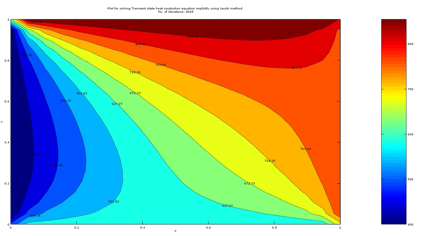
Number of iterations done are 8045
Time taken for solving equation is 0.079604
2.Gauss Seidel Unsteady Implicit
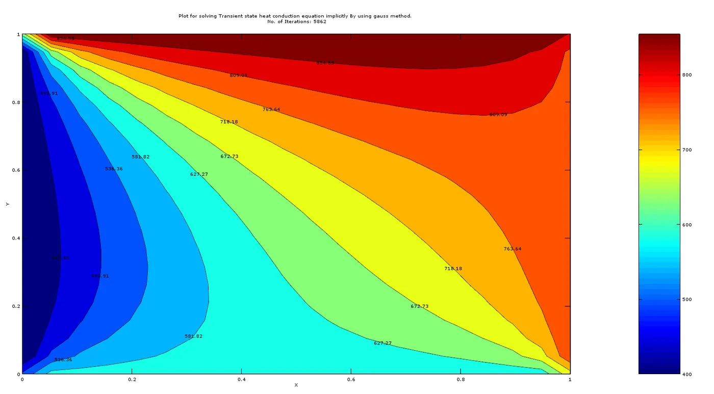
Number of iterations done are 5862
Time taken for solving equation is 0.058604
3.SOR Unsteady Implicit
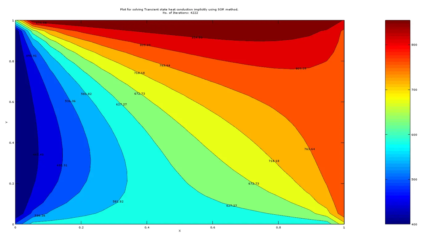
Relaxation Factor 1.729454
Number of iterations done are 4222
Time taken for solving equation is 0.047837
conclusion
The SOR method converges the solution even faster as we can see that for the same number of iterations the final temperature distribution is even further. This is because of the extra term in conjunction with the Gauss Siedel term which helps in converging the solution faster. Also the value of relaxation parameter largely affects the convergence criteria.
Final Observation:
Following are the some important points inferences:
1. The unsteady state equations can be solved both Explicitly and Implicitly where as the Steady State equations can only be solved Implicitly.
2. Talking in general out of the Three Iterative Solvers the SOR is the best option as it converges the solution faster and also with very high accuracy.
3. The choice of the Iterative Solver largely depends upon the Differential Eqaution as well as the Boundary Conditons. As in the case we saw that SOR method took greater time to solve the transient equation than the two other solvers.