Simulation of Flow through a pipe in OpenFoam
Hagen- Poiseuille's Equation
Hagen Poiseuille states that for a specified flow rate, the pressure drops and thus the required pumping power is proportional to the length of the pipe and the viscosity of the fluid, but it is inversely proportional to the fourth power of the radius (or diameter) of the pipe. Therefore, the pumping power requirement for a laminar-flow piping system can be reduced by a factor of 16 by doubling the pipe diameter.
ΔP=8μLQ/πR4
where,
ΔP= pressure difference between the two ends,
L= length of pipe,
μ= dynamic viscosity,
Q= volumetric flow rate,
π= pi,
R= pipe radius
Reynold's Number:
The transition from laminar to turbulent flow depends on the geometry, surface roughness, flow velocity, surface temperature, and type of fluid, among other things. After exhaustive experiments in the 1880s, Osborne Reynolds discovered that the flow regime depends mainly on the ratio of inertial forces to viscous forces in the fluid. This ratio is known as Reynold's number and is given as:
Re=(ρ(Vavg^2)(L^2))/(μVavgL)=(ρVavgL)/μ=(VavgL)/ν
where,
Vavg - Average velocity of the fluid
D - Characteristic Length of the flow domain (in this case, diameter)
ρ - density of fluid
μ - Dynamic viscosity
υ - Kinematic viscosity
The value of Reynold's number gives us a general idea whether the flow is laminar or turbulent. Generally, a flow with Re < 2300 is said to be laminar and a flow with Re > 4000 is said to be turbulent. The flow with Re ranging in between is said to be transitional. Reynold's number gives a fair idea of the flow in quotidian physical conditions. A flow with Re 100,000 can also be maintained laminar under conditions of very smooth pipes and avoiding any vibrational and flow disturbances.
Laminar Flow
Laminar or streamline flow in pipes (or tubes) occurs when a fluid flows in parallel layers, with no disruption between the layers. At low velocities, the fluid tends to flow without lateral mixing, and adjacent layers slide past one another. There are no cross-currents perpendicular to the direction of flow, nor eddies or swirls of fluids. In laminar flow, the motion of the particles of the fluid is very orderly with all particles moving in straight lines parallel to the pipe walls. Any lateral mixing (mixing at right angles to the flow direction) occurs by the action of diffusion between layers of the liquid. Diffusion mixing can be slow however if the diameter of the pipe of the tube is small then this diffusive mixing can be very significant.
Turbulent Flow
Turbulent flow is a flow regime characterized by chaotic property changes. This includes a rapid variation of pressure and flows velocity in space and time. Turbulent flow is a type of fluid (gas or liquid) flow in which the fluid undergoes irregular fluctuations, or mixing, in contrast to laminar flow, in which the fluid moves in smooth paths or layers. In turbulent flow, the speed of the fluid at a point is continuously undergoing changes in both magnitude and direction.
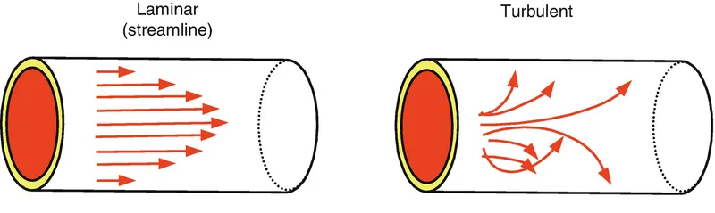
Most kinds of fluid flow are turbulent, except for laminar flow at the leading edge of solids moving relative to fluids or extremely close to solid surfaces, such as the inside wall of a pipe, or in cases of fluids of high viscosity (relatively great sluggishness) flowing slowly through small channels. Common examples of turbulent flow are blood flow in arteries, oil transport in pipelines, lava flow, atmosphere and ocean currents, the flow through pumps and turbines, and the flow in boat wakes and around aircraft-wing tips.
Entrance Region:
Consider a fluid entering a circular pipe at a uniform velocity. Because of the no-slip condition, the fluid particles in the layer in contact with the surface of the pipe come to a complete stop. This layer also causes the fluid particles in the adjacent layers to slow down gradually as a result of friction. To make up for this velocity reduction, the velocity of the fluid at the midsection of the pipe has to increase to keep the mass flow rate through the
pipe constant. As a result, a velocity gradient develops along the pipe.
The region of the flow in which the effects of the viscous shearing forces caused by fluid viscosity are felt is called the velocity boundary layer or just the boundary layer. The hypothetical boundary surface divides the flow in a pipe into two regions: the boundary layer region, in which the viscous effects and the velocity changes are significant, and the irrotational (core) flow region, in which the frictional effects are negligible and the velocity remains essentially constant in the radial direction.
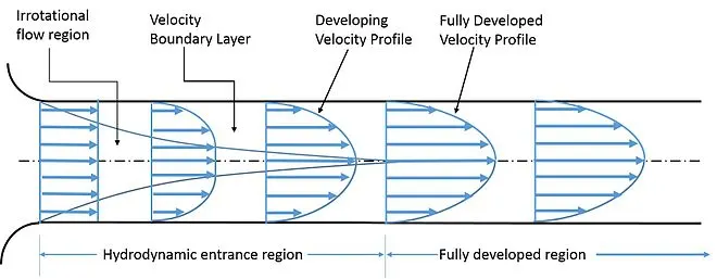
Velocity boundary layer development in a pipe
The thickness of this boundary layer increases in the flow direction until the boundary layer reaches the pipe center and thus fills the entire pipe. The region from the pipe inlet to the point at which the boundary layer merges at the centerline is called the hydrodynamic entrance region, and the length of this region is called the hydrodynamic entry length Lh. Flow in the entrance region is called hydrodynamically developing flow since this is the region where the velocity profile develops. The region beyond the entrance region in which the velocity profile is fully developed and remains unchanged is called the hydrodynamically fully developed region. The flow is said to be fully developed when the normalized temperature profile remains unchanged as well.
The hydrodynamic entry length is usually taken to be the distance from the pipe entrance to where the wall shear stress (and thus the friction factor) reaches within about 2% of the fully developed value.
For Laminar Flow
Lh,laminar/D=0.05Re
Velocity Profile for Laminar Flow through Pipe
The velocity profile in a fully developed laminar flow in a pipe is parabolic with a maximum at the centerline and a minimum (zero) at the pipe wall. Also, the axial velocity u is positive for any r, and thus the axial pressure gradient dP/dx must be negative that is the pressure must decrease in the flow direction because of viscous effects—it takes pressure to push the fluid through the pipe.
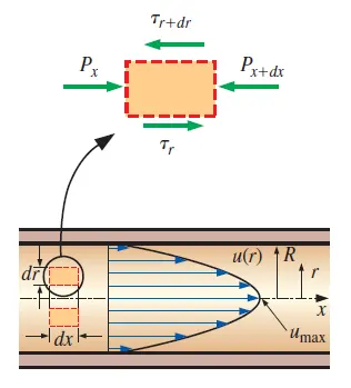
u(r)=−((R^2)/4μ)(dp/dx)(1−(r^2)/(R^2))
u(r)=2Vavg(1−(r^2)/(R^2))
The velocity profile since Vavg can be determined easily from the flow rate information. The maximum velocity occurs at the centerline and is determined by substituting r=0.
umax=2Vavg
The average velocity in fully developed laminar pipe flow is one-half of the maximum velocity.
The fluid velocity in a pipe changes from zero at the wall because of the no-slip condition to a maximum at the pipe centre. In fluid flow, it is convenient to work with an average velocity Vavg, which remains constant in incompressible flow when the cross-sectional area of the pipe is constant.
Pressure Drop
A quantity of interest in the analysis of pipe flow is the pressure drop ΔP since it is directly related to the power requirements of the fan or pump to maintain flow.
ΔP=P2−P1
dP/dx=(P2−P1)/L
A pressure drop due to viscous effects represents an irreversible pressure loss.
Head Loss
The head loss hL represents the additional height that the fluid needs to be raised by a pump in order to overcome the frictional losses in the pipe.
hL=ΔPL/ρg
Problem statement
For flow in pipe of diameter D, experimental observations shows that for “fully developed” flow, laminar flow occurs when ReD< 2300. Therefore, let us consider Re for flow is 2100. Assume diameter of pipe (D)=0.02m , also consider working fluid as water at temperature 25 degree Celcious so the values of density (ρ)=997kg/m^3 and Dynamic Viscosity (μ)=0.00089 Pa.s and Kinematic Viscosity (υ) = 8.927*10^-7 m^2/s
Hence given properties are as follows:
Reynold's Number (Re) = 2100
Pipe Diameter (D) = 0.02m
Entry Length (Le) = 0.05*Re*D = 2.1m
Pipe length (L) = 2.6m (0.5 meter extra for fully developed flow profile)
Density of water (ρ) = 997 kg/m^3
Dynamic Viscosity (μ) = 0.0008891 Pa.s
Kinematic Viscosity (υ) = 8.917e-7 m^2/s
Analytical Values:
Average Velocity
(Vavg) = (Re*μ) / (ρ*D) = (2100*0.00089)/(997*0.02) = 0.09373 m/s
Maximum Velocity
(Vmax) = 2*Vavg = 2*0.09373 = 0.187463 m/s
Pressure Drop
(dP)=(32*μ*L*Vavg)/(D^2)=(32*0.00089*3.1*0.09373)/(0.02^2)=20.688 Pa
Kinematic Pressure Drop
(dPk) = dP/ρ = 20.688/997 = 0.02m
Pre-processing
In order to start the simulation process, First start terminal in Linux Operating system using ctrl+alt+T buttons on key board or right click -> Open Terminal. After starting terminal yo will see following window.
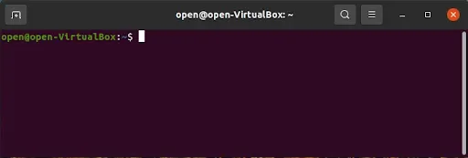
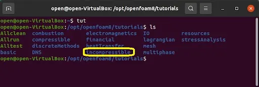
Now, we have to simulate our problem in openFOAM and we are going to solve our problem using tutorials present in openFOAM, therefore, just type ‘tut’ to open OpenFOAM tutorial directory. And type ‘ls’ to identify what kind of tutorials present inside this directory.
We have to solve incopressible flow simulation for this problem so select incompressible directory by typing 'cd incompressible' and then again type 'ls' to explore folders in incopressible folders.
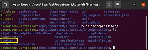
In above picture, we can see the plethora of solver folders. For this particular solver we need solver for laminar-viscous flow. So here we choose 'icoFoam'
icoFoam is the solver in openFoam which is use as transient solver for incopressible, laminar flow of Newtonian fluids.
(Newtonian fluid is a fluid in which the viscous stress arising from its flow, at every point, are linearly correlated to the local strain rate - the rate of change of its deformation over time. Newtonian fluids are the simplest mathematical models of fluids that account for viscosity.)
Therefore, we will select icoFoam folder by typing 'cd icoFoam' and by typing 'ls' we explore this folder in terminal.
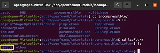
Here, we have, again to option, cavity and elbow. They both are part of the icoFoam solver and cavity section use to create required domain and black mesh so select 'cavity' folder.
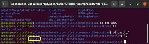
In cavity, we are, again, going to see cavity folder, where we have to define our fluid domain and generate block mesh.
But we are not going to make any changes here in tutorial section. First of all, OpenFoam does no let anyone make any changes in their official tutorial and secondly, any changes with their official tutorials my corrupt openFoam. An in a bid to correct it, we may need to reinstall open foam all over again.
So, we are going to copy this cavity folder using 'cp -r cavity' command. Next, rename it as ‘cavtest’ and paste it in openFoam run folder by typing 'cp -r cavity $FOAM_RUN/cavtest'.
And then open run folder by typing 'cd $FOAM_RUN'. where we can see 'cavtest' file.
Now, we can make any changes to the cavtest file, which will never affect the openFoam official files. Open cavtest folder. Here, we can provide specification for our block mesh in system folder.
Geometry Generation:
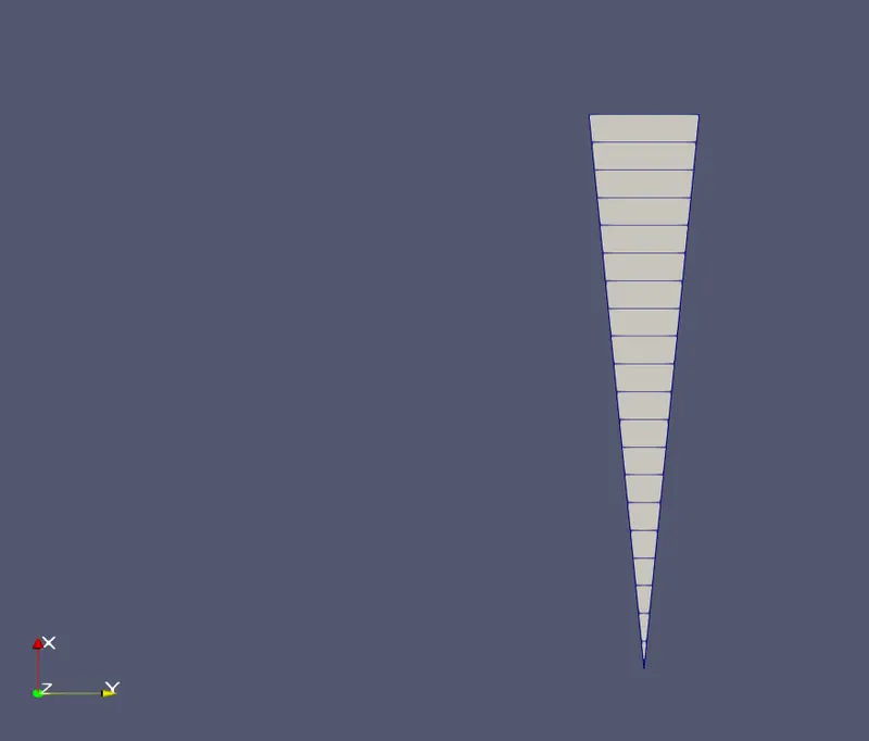
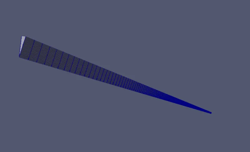
Modelling and simulating flow through an entire pipe in OpenFoam takes high computing power. Hence, a small wedge section of the pipe was modelled with a wedge angle of 4 degrees.
The blockMeshDict file required was written using MATLAB code by file parsing techniques..
MATLAB Code:
close all
clear all
clc

%Given Inputs
re=2100;    %Reynolds Number

%Assumptions
d=0.02;   %Diamter of the Pipe
r=d/2;      %Radius of the Pipe

%theta_f=input(Enter Wedge Angle Less Than 5°=);
theta=4;

% Numerical Analysis OF Entry Length for Laminar Flow
l_e=0.05*re*d;  %flow direction

%Total Lenght Of Pipe
l=l_e+0.5; %Assuming 0.5m extra for fully developed flow profile

%Finding the coordinates for the wedge
y=r*sind(theta);  %y-direction

x=r*cosd(theta);  %x-direction

% Points
point0=[0 0 0]; %0
point1=[x y 0]; %1
point4=[x -y 0]; %4
point3=[0 0 l]; %3
point2=[x y l]; %2
point5=[x -y l]; %5

%Creating the blockMeshDict File
f= fopen('blockMeshDict.txt','w');

fprintf(f,'%sn','/*--------------------------------*- C++ -*----------------------------------*');
fprintf(f,'%sn','  =========                 |');
fprintf(f,'%sn','  \      /  F ield         | OpenFOAM: The Open Source CFD Toolbox');
fprintf(f,'%sn','   \    /   O peration     | Website:  https://openfoam.org');
fprintf(f,'%sn','    \  /    A nd           | Version:  8');
fprintf(f,'%sn','     \/     M anipulation  |');
fprintf(f,'%sn','*---------------------------------------------------------------------------*/');
fprintf(f,'%sn','FoamFile');
fprintf(f,'%sn','{');
fprintf(f,'%sn','    version     2.0;');
fprintf(f,'%sn','    format      ascii;');
fprintf(f,'%sn','    class       dictionary;');
fprintf(f,'%sn','    object      blockMeshDict;');
fprintf(f,'%sn','}');
fprintf(f,'%sn','// * * * * * * * * * * * * * * * * * * * * * * * * * * * * * * * * * * * * * //');
fprintf(f,'%sn','');
fprintf(f,'%sn','convertToMeters 1;');

fprintf(f,'%sn','');


fprintf(f,'%sn','vertices');
fprintf(f,'%sn','(');
fprintf(f,'    (%f %f %f)n',point0(1),point0(2),point0(3));
fprintf(f,'    (%f %f %f)n',point1(1),point1(2),point1(3));
fprintf(f,'    (%f %f %f)n',point2(1),point2(2),point2(3));
fprintf(f,'    (%f %f %f)n',point3(1),point3(2),point3(3));
fprintf(f,'    (%f %f %f)n',point4(1),point4(2),point4(3));
fprintf(f,'    (%f %f %f)n',point5(1),point5(2),point5(3));
fprintf(f,'%sn',');');

fprintf(f,'%sn','');

fprintf(f,'%sn','blocks');
fprintf(f,'%sn','(');
fprintf(f,' %sn','hex (0 4 1 0 3 5 2 3) (10 1 750) simpleGrading (1 1 1)');
fprintf(f,'%sn',');');

fprintf(f,'%sn','');

fprintf(f,'%sn','edges');
fprintf(f,'%sn','(');
fprintf(f,' arc 1 4 (%f 0 0)n',r);
fprintf(f,' arc 2 5 (%f 0 %f)n',r,l);
fprintf(f,'%sn',');');

fprintf(f,'%sn','');

fprintf(f,'%sn','boundary');
fprintf(f,'%sn','(');

fprintf(f,' %sn','front');
fprintf(f,' %sn','{');
fprintf(f,'  %sn','type wedge;');
fprintf(f,'  %sn','faces');
fprintf(f,'  %sn','(');
fprintf(f,'   %sn','(0 1 2 3)');
fprintf(f,'  %sn',');');
fprintf(f,' %sn','}');

fprintf(f,' %sn','back');
fprintf(f,' %sn','{');
fprintf(f,'  %sn','type wedge;');
fprintf(f,'  %sn','faces');
fprintf(f,'  %sn','(');
fprintf(f,'   %sn','(0 3 5 4)');
fprintf(f,'  %sn',');');
fprintf(f,' %sn','}');

fprintf(f,' %sn','tankwall');
fprintf(f,' %sn','{');
fprintf(f,'  %sn','type wall;');
fprintf(f,'  %sn','faces');
fprintf(f,'  %sn','(');
fprintf(f,'   %sn','(1 4 5 2)');
fprintf(f,'  %sn',');');
fprintf(f,' %sn','}');

fprintf(f,' %sn','inlet');
fprintf(f,' %sn','{');
fprintf(f,'  %sn','type patch;');
fprintf(f,'  %sn','faces');
fprintf(f,'  %sn','(');
fprintf(f,'   %sn','(0 4 1 0)');
fprintf(f,'  %sn',');');
fprintf(f,' %sn','}');

fprintf(f,' %sn','outlet');
fprintf(f,' %sn','{');
fprintf(f,'  %sn','type patch;');
fprintf(f,'  %sn','faces');
fprintf(f,'  %sn','(');
fprintf(f,'   %sn','(3 5 2 3)');
fprintf(f,'  %sn',');');
fprintf(f,' %sn','}');

fprintf(f,' %sn','axis');
fprintf(f,' %sn','{');
fprintf(f,'  %sn','type empty;');
fprintf(f,'  %sn','faces');
fprintf(f,'  %sn','(');
fprintf(f,'   %sn','(0 3 3 0)');
fprintf(f,'  %sn',');');
fprintf(f,' %sn','}');

fprintf(f,'%sn',');');


fprintf(f,'%sn','');

fprintf(f,'%sn','mergePatchPairs');
fprintf(f,'%sn','(');
fprintf(f,'%sn',');');
fprintf(f,'%sn','');
fprintf(f,'%sn','// ************************************************************************* //');

fclose(f);
After running above codes, we will get our BlockMeshDict file as output.
/*--------------------------------*- C++ -*----------------------------------*
  =========                 |
  \      /  F ield         | OpenFOAM: The Open Source CFD Toolbox
   \    /   O peration     | Website:  https://openfoam.org
    \  /    A nd           | Version:  8
     \/     M anipulation  |
*---------------------------------------------------------------------------*/
FoamFile
{
    version     2.0;
    format      ascii;
    class       dictionary;
    object      blockMeshDict;
}
// * * * * * * * * * * * * * * * * * * * * * * * * * * * * * * * * * * * * * //

convertToMeters 1;

vertices
(
    (0.000000 0.000000 0.000000)
    (0.009976 0.000698 0.000000)
    (0.009976 0.000698 2.600000)
    (0.000000 0.000000 2.600000)
    (0.009976 -0.000698 0.000000)
    (0.009976 -0.000698 2.600000)
);

blocks
(
 hex (0 4 1 0 3 5 2 3) (10 1 750) simpleGrading (1 1 1)
);

edges
(
 arc 1 4 (0.010000 0 0)
 arc 2 5 (0.010000 0 2.600000)
);

boundary
(
 front
 {
  type wedge;
  faces
  (
   (0 1 2 3)
  );
 }
 back
 {
  type wedge;
  faces
  (
   (0 3 5 4)
  );
 }
 tankwall
 {
  type wall;
  faces
  (
   (1 4 5 2)
  );
 }
 inlet
 {
  type patch;
  faces
  (
   (0 4 1 0)
  );
 }
 outlet
 {
  type patch;
  faces
  (
   (3 5 2 3)
  );
 }
 axis
 {
  type empty;
  faces
  (
   (0 3 3 0)
  );
 }
);

mergePatchPairs
(
);

// ************************************************************************* //
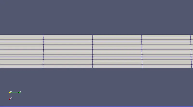
Copy above blockMeshDict file and replace it in the system directory of the pipe folder and by running this block mesh file we will get following mesh:
Furthermore, we are going to edit ‘controlDict’ file to provides time limits - start time and end time. Also to represent deltat. While selection of deltat CFL value shoud be less than 1. otherwise, the solution could stopped forcibly or it may diverge at the time of converging. So make following changes in ‘controlDict’ file.
controlDict
/*--------------------------------*- C++ -*----------------------------------*
  =========                 |
  \      /  F ield         | OpenFOAM: The Open Source CFD Toolbox
   \    /   O peration     | Website:  https://openfoam.org
    \  /    A nd           | Version:  8
     \/     M anipulation  |
*---------------------------------------------------------------------------*/
FoamFile
{
    version     2.0;
    format      ascii;
    class       dictionary;
    location    "system";
    object      controlDict;
}
// * * * * * * * * * * * * * * * * * * * * * * * * * * * * * * * * * * * * * //

application     icoFoam;

startFrom       startTime;

startTime       0;

stopAt          endTime;

endTime         5;

deltaT          1e-2;

writeControl    timeStep;

writeInterval   100;

purgeWrite      2;

writeFormat     ascii;

writePrecision  6;

writeCompression off;

timeFormat      general;

timePrecision   6;

runTimeModifiable true;


// ************************************************************************* //
Boundary and initial conditions
Then, we have to define initial value for pressure and velocity. In order to do that, we have to go back in cavity_copy directory using ‘cd ..’ command and select folder named ‘0’, which stand for initial values. In this case initial value for pressure and velocity.
When solving circulating internal flow, the most common boundary conditions are to fix an inlet velocity and an outlet pressure.
Initial setting for pressure
/*--------------------------------*- C++ -*----------------------------------*
  =========                 |
  \      /  F ield         | OpenFOAM: The Open Source CFD Toolbox
   \    /   O peration     | Website:  https://openfoam.org
    \  /    A nd           | Version:  8
     \/     M anipulation  |
*---------------------------------------------------------------------------*/
FoamFile
{
    version     2.0;
    format      ascii;
    class       volScalarField;
    object      p;
}
// * * * * * * * * * * * * * * * * * * * * * * * * * * * * * * * * * * * * * //

dimensions      [0 2 -2 0 0 0 0];

internalField   uniform 0;

boundaryField
{
    inlet
    {
        type            zeroGradient;
    }

    outlet
    {
        type            fixedValue;
        value		 uniform 0;
    }

    front
    {
        type            wedge;
    }

    back
    {
	type		wedge;
    }

    tankWall
    {
	type		zeroGradient;
    }

    axis
    {
    	type		empty;
    }
}


// ************************************************************************* //
In the U dictionary one can find out a new type of boundary condition: inlet and outlet. It switches U and p between fixedValue and zeroGradient: the first when the flow is in-going and the second when it is outgoing.
Example: in circular pipe case, the outlet velocity will always be adapted to the conditions according to zeroGradient except if there is an inflow at the outlet patch. If this happens, to this inflow velocity it is assigned the value specified under the inletOutlet instruction and so the flow will always be outgoing.
Initial setting for Velocity
/*--------------------------------*- C++ -*----------------------------------*
  =========                 |
  \      /  F ield         | OpenFOAM: The Open Source CFD Toolbox
   \    /   O peration     | Website:  https://openfoam.org
    \  /    A nd           | Version:  8
     \/     M anipulation  |
*---------------------------------------------------------------------------*/
FoamFile
{
    version     2.0;
    format      ascii;
    class       volVectorField;
    object      U;
}
// * * * * * * * * * * * * * * * * * * * * * * * * * * * * * * * * * * * * * //

dimensions      [0 1 -1 0 0 0 0];

internalField   uniform (0 0 0);

boundaryField
{

    axis

    {

	type		empty;

    }


    inlet

    {

        type            fixedValue;

        value           uniform (0 0 0.09373);

    }


    outlet

    {

        type            zeroGradient;

    }


    front

    {

        type            wedge;

    }


    back

    {

	type		wedge;

    }


    tankWall

    {

        type            fixedValue;

        value           uniform (0 0 0);

    }

}

// ************************************************************************* //
Next, we have to mention dynamic viscosity in transportProperty in constant directory of the Pipe.
transportProperty
/*--------------------------------*- C++ -*----------------------------------*
  =========                 |
  \      /  F ield         | OpenFOAM: The Open Source CFD Toolbox
   \    /   O peration     | Website:  https://openfoam.org
    \  /    A nd           | Version:  8
     \/     M anipulation  |
*---------------------------------------------------------------------------*/
FoamFile
{
    version     2.0;
    format      ascii;
    class       dictionary;
    location    "constant";
    object      transportProperties;
}
// * * * * * * * * * * * * * * * * * * * * * * * * * * * * * * * * * * * * * //

nu              [0 2 -1 0 0 0 0] 8.917e-7;


// ************************************************************************* //
After deploying mesh, now we are ready to run the simulation. Simulation that we selected was icoFoam. Hence, just type ‘icoFoam’ and simulation will start.
Post-processing
Now, let us view the results in paraView by using ‘paraFoam’ command
Velocity Profile:
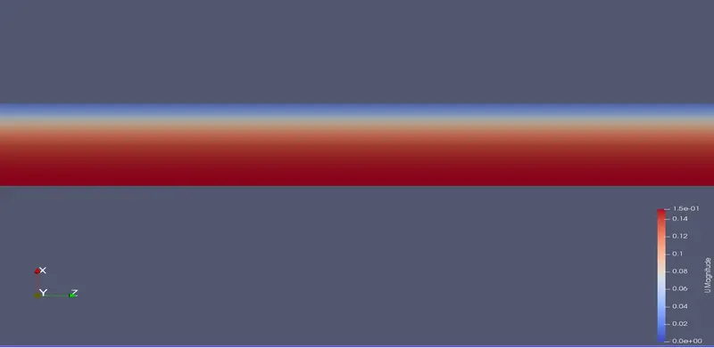
velocity profile (middle)
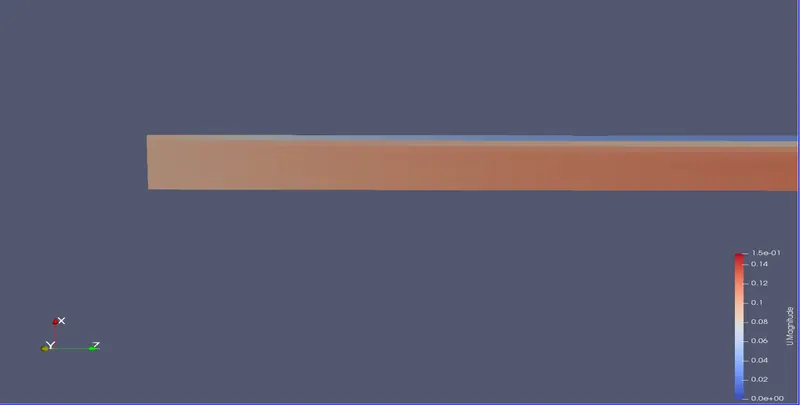
velocity profile (at the inlet, shear force increasing as the fluid is moving forward)
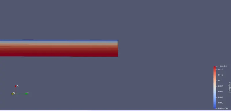
velocity profile (at the outlet, shear stress and velocity stable as it reaches the end)
Pressure Distribution:
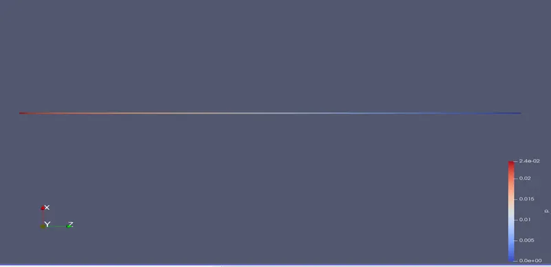
(left -p at inlet, right- p at outlet; the pressure at the beginning is high and as fluid is moving forward through pipe its decreasing.The pressure is lowest at the end of pipe)
Velocity profile at distance 2.5m and 0.01m (from the inlet of pipe, 0.1m, and comparison of it with fully developed velocity flow, 2.5m)
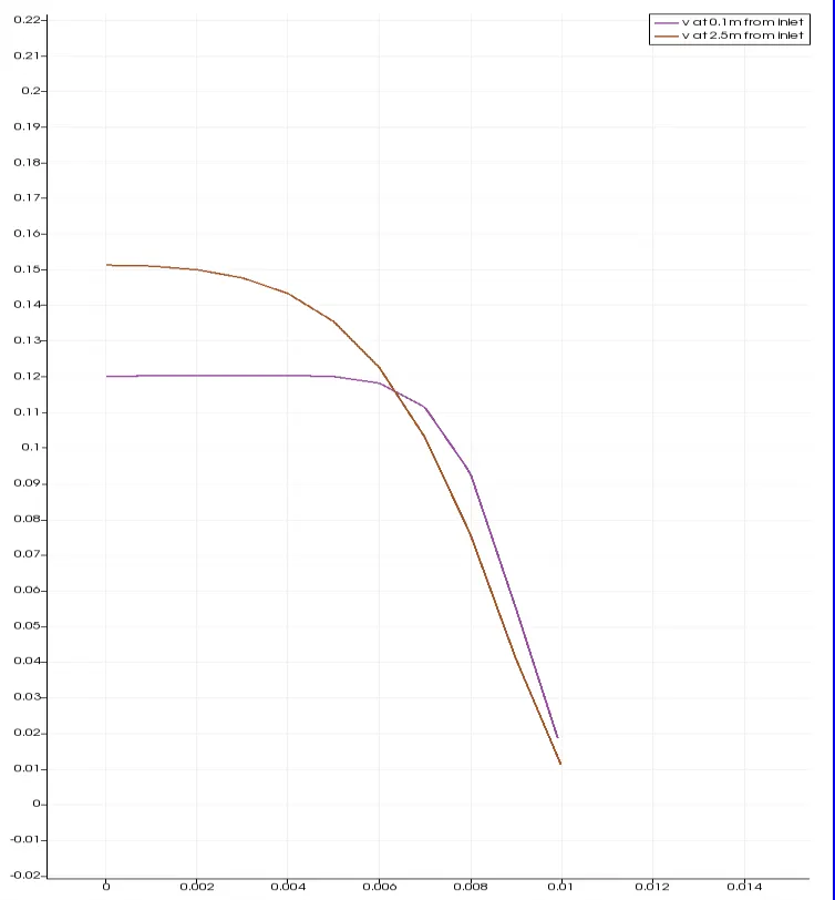
So we can observe that as water moving forward through pipe its velocity profile along the radius of pipe is stabilizing and there is a point within a length of point where it does not change that point is call fully developed flow region. And it comes after entrance length which we calculated in above section of this project.
Pressure change along the length of pipe
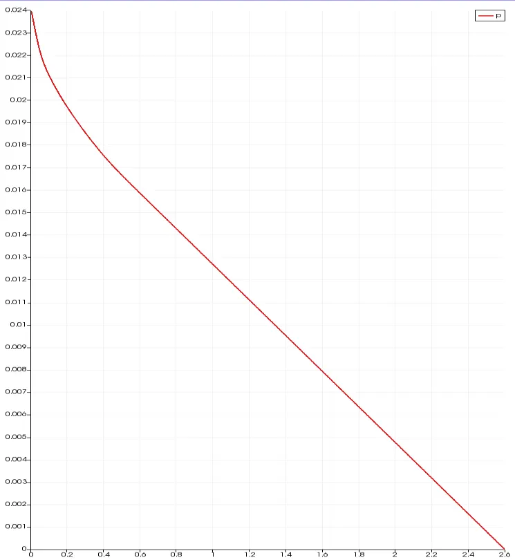
If we check the pressure plot along the length of the pipe its gradually decreasing as the velocity increasing.
Shear Stress :-
shear stress = (dynamic Viscosity)*(du/dy)
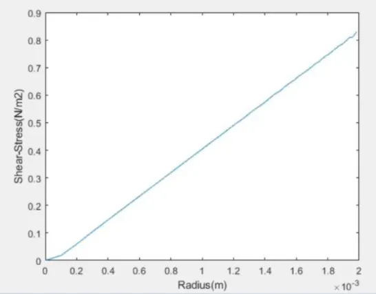
If we focus on shear stress along radius of the pipe, in fully developed flow region, we can observe there is very less shear stress at the center as there is no wall is present to restrict the flow of fluid. But from center to wall the, we can see, the shear stress increasing gradually and its value near the wall is maximum.
Conclusion:-
- Validated Hydro-dynamic length with the numerical result.
- Validated the fully developed flow velocity profile with its analytical profile.
- Validated maximum velocity and pressured drop for fully developed flow.
- Post-processed Shear stress and validated wall shear stress for fully developed flow.