Week - 8 Mass Scaling

Mass Scaling

Aim

• To understand the effect of mass scaling on simulation run time and stability in Ls Dyna
• The difference in the explicit and implicit analysis of the same simulation

Theory

Mass-scaling refers to a technique whereby nonphysical mass is added to a structure to achieve a larger explicit timestep.

Anytime you add nonphysical mass to increase the timestep in a dynamic analysis, you affect the results (think of F=m*a). Sometimes the effect is insignificant and in those cases adding nonphysical mass is justifiable. Examples of such cases may include the addition of mass to just a few small elements in a noncritical area or quasi-static simulations where the velocity is low and the kinetic energy is very small relative to the peak internal energy. In the end, it's up to the judgement of the analyst to gauge the effect of mass scaling. You may have to reduce or eliminate mass scaling in a second run to gauge the sensitivity of the results to the amount of mass added.

One can selectively employ mass scaling by artificially increasing the material density of the parts you want to mass-scale. This manual form of mass scaling is done independently of the automatic mass scaling invoked with DT2MS in *CONTROL_TIMESTEP.

When DT2MS is input as a negative value, mass is added only to those elements whose timestep would otherwise be less than
|DT2MS|. By adding mass to these elements, their timestep becomes equal to |DT2MS|. An infinite number of combinations of TSSFAC and DT2MS will give the same product, i.e., timestep but the added mass will be different for each of those combinations. The trend is that the bigger |DT2MS| (and the smaller TSSFAC while TSSFAC*|DT2MS|=const), the greater the added mass. In return, stability may improve as TSSFAC is reduced (just as in non-mass-scaled solutions). If stability is a problem with the default TSSFAC of 0.9, try 0.8 or 0.7. If you reduce TSSFAC, you can increase |DT2MS| proportionally so that their product, and hence timestep, is unchanged.

To determine where and when mass is automatically added, write GLSTAT and MATSUM files. These files will allow you to plot added mass vs. time for the complete model and individual parts, respectively. To produce fringe plots of added mass in parts comprised of shell elements (DT2MS negative), set STSSZ=3 in *DATABASE_EXTENT_BINARY. You can then fringe the added mass (per element) using LS-POST by choosing Fcomp > Misc > time step size. (Here, the label "time step size" is the element added mass.)

The difference between using a positive or negative number for DT2MS in*CONTROL_TIMESTEP is as follows:

Negative: Mass is added to only those elements whose timestep would otherwise be less than TSSF*abs(DT2MS). When mass scaling is appropriate, this method is recommended.

Positive: Mass is added or taken away from elements so that the timestep of every element is the same. There is no advantage to using this method over the negative DT2MS method.

The parameter MS1ST in *CONTROL_TIMESTEP controls whether the mass is added only once during initialization (MS1ST=1) or anytime as necessary to maintain the desired timestep specified via DT2MS (MS1ST=0).

You can use ENDMAS in *CONTROL_TERMINATION to stop the calculation after a certain amount of mass has been added (active for automatic mass scaling only).

Mass-scaling of deformable spotweld beams:

The mass-scaling parameter in *MAT_SPOTWELD (DT) affects only the spot welds. If no mass-scaling is invoked in *CONTROL_TIMESTEP (DT2MS=0.) AND the timestep is controlled by the deformable spot welds, DT can be used to add inertia to the spot welds during initialization to increase the timestep to a value of DT. When DT is nonzero, mass added to spotweld beams is reported to d3hsp. MATSUM momentum and KE does NOT factor in added mass to def. spotwelds. GLSTAT DOES factor in added mass to total KE.

Consider 3 cases of invoking mass-scaling in a model with deformable spot welds:

1. Although "percentage mass increase" under "Deformable Spotwelds:" in d3hsp is bogus when DT2MS is neg. and DT in *MAT_SPOTWELD = 0, the following are correct: "added spotweld mass" in d3hsp "added mass" and "percentage increase" in d3hsp AFTER the first time step "added mass" in glstat and matsum
2. Added spotweld mass controlled by DT in *MAT_SPOTWELD is NOT INCLUDED in "added mass" given in d3hsp, glstat, or matsum when DT2MS is neg. and DT in *MAT_SPOTWELD is nonzero. This can be quite misleading. The user must check for "added spotweld mass" in d3hsp. Recommended: Do not invoke both mass-scaling criteria. Neg. DT2MS with DT=0 (case 1 above) is preferred.
3. If DT is nonzero and DT2MS=0, the initial timestep will NOT consider added spotweld mass but the time step will increase by 10% each cycle until the correct timestep (considering added spotweld mass) is achieved. Glstat and matsum contain no "added mass" line item.

Selective mass-scaling:

Selective mass-scaling (new in LS-DYNA V971 R3) is invoked using DT2MS and IMSCL in *CONTROL_TIMESTEP. Selective mass-scaling can be turned on using the IMSCL in *CONTROL_TIMESTEP and could apply either to all the parts of the model (set to 1) or do just a few parts (<0 with abs(IMSCL) = part set list) which is recommended as the selective mass-scaling is both memory and CPU intensive.

The selective mass scaling option requires the solving of a sparse equation system every time step. The mass matrix is no longer diagonal. Storing the non-diagonal mass matrix requires some memory and the solution of m*a=F takes some CPU time. The system is solved iteratively.

The following entities are not affected by mass scaling:

• Thermal solution response in a fully coupled thermal-stress analysis
• Gravity loads, viscous pressure loads
• Adiabatic heat calculations
• Equation of state materials
• Fluid and fluid link elements
• Surface-based fluid cavities
• Spring and dashpot elements

Procedure

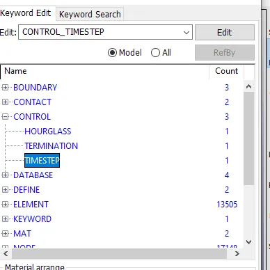
• Open the file in ls prepost and check the Control Timestep card.

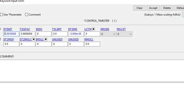
• Run this as the default simulation and note the runtime and added mass.

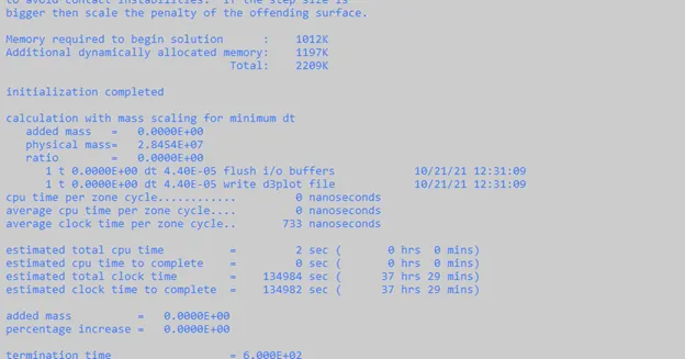
The run time is 37hrs and 29 mins.

• Changing the value of DT2MS to -6.5e^-5 and run the simulation

Iteration 1: DT2MS=-6.5 e^-05

The total clock time has been reduced to 18 hours and 54mins with a mass percentage increase of 0.057%

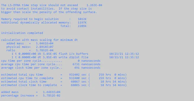
Changing the timescale factor to 0.7. The product of TTSFAC and DT2MS is reduced, thereby it can be concluded that they directly affect run time as the CPU time is significantly more in this case.

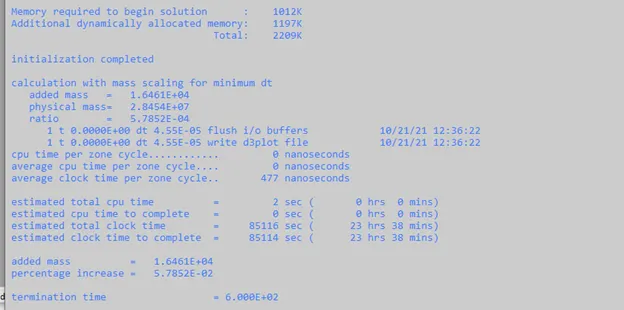
Iteration 2

Set Scalefactor back to 0.9 and change DT2MS to -8.5e^-05

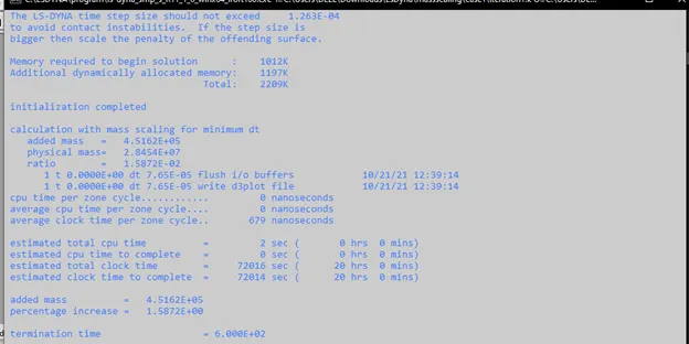
Iteration 3

Changing the value of DT2MS to -11.5e^-05

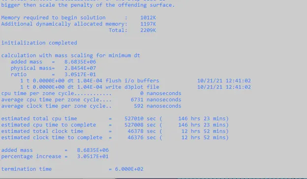
Iteration 4

Changing the value of DT2MS to 10.5e^-05

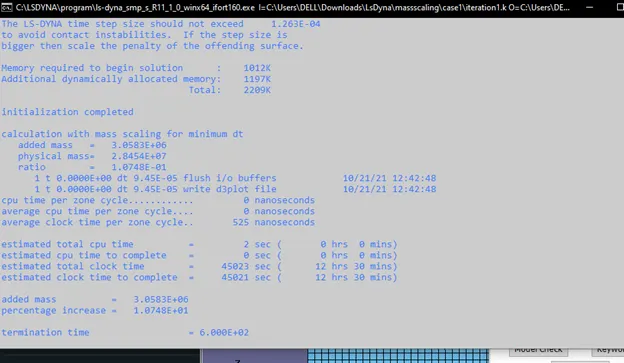
Iteration 5

Changing the value of DT2MS to -10.3e^-05

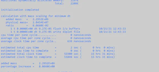
At TSSFAC of 0.9 and DT2MS of -10.3e^-05, a percentage increase of 8% has been observed.

DT2MS xe-05	Time Seconds	Mass Percentage %
-3.5	134984	0
-6.5	68067	0.05
-8.5	72016	1.58
-11.5	46376	30.5
-10.5	45021	10.7
-10.3	55898	8.066

Plotting the histogram chart to visualize the difference in time taken for each iteration.

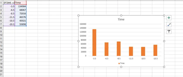
It can be observed that mass scaling can significantly decrease computational time. We limit ourselves to a maximum mass added per cent of 8 so that it doesn’t drastically change the results.

Implicit

Add the control implicit auto, general, solver and solution cards.

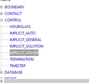
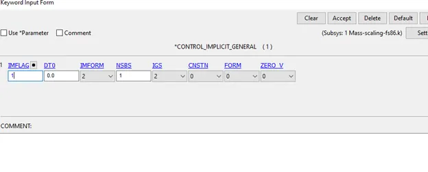
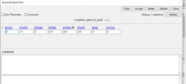
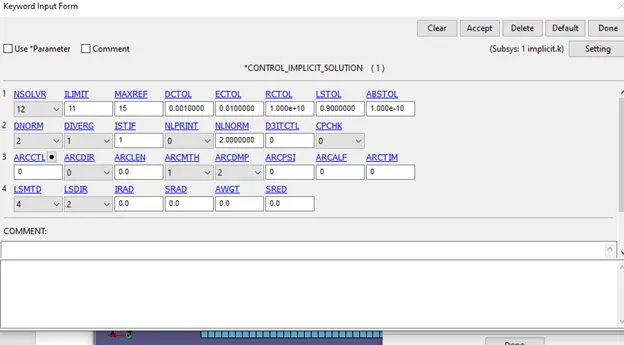
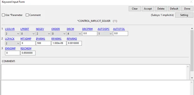
Run the simulation after

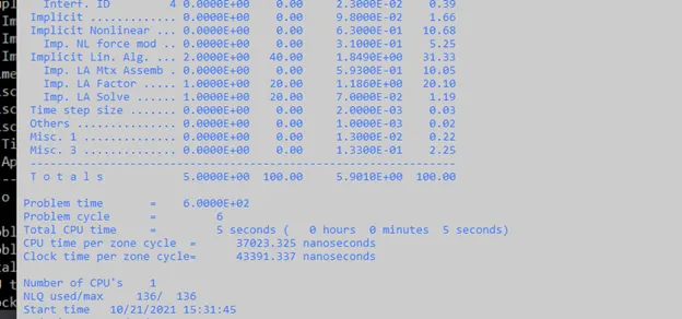
It can be seen that implicit analysis solves it instantly, this is because in Implicit Analysis Timestep does not need to be smaller than courant timestep due to the stability of implicit solutions. This is why there is a huge difference in the time taken for explicit and implicit analysis for the same case.

Learning Outcomes

• Mass scaling in ls dyna

Conclusion

Mass scaling enables an analysis to be performed economically without artificially increasing the loading rate. Mass scaling is the only option for reducing the solution time in simulations involving a rate-dependent material or rate-dependent damping, such as dashpots. In such simulations increasing the loading rate is not an option because material strain rates increase by the same factor as the loading rate. When the properties of the model change with the strain rate, artificially increasing the loading rate artificially changes the process.

In this project, the effect of mass scaling on the computational time of an FEA simulation was observed.It can be concluded that mass scaling can greatly reduce the computational cost of an Explicit FEA simulation.The percentage of mass added has been limited to 8% so as to not drastically effect the results of the simulation.the time step in an explicit finite element analysis must be less than the Courant Time Step (i.e., the time taken by a sound wave to travel across an element) while implicit analyses have no such limitations. This is why there is a huge difference in the time taken for explicit and implicit analysis for the same case, as there are no such limitations to timestep in implicit analysis due to the unconditional stability of implicit methods.