Mass Scaling Using LS-DYNA
INTRODUCTION
Mass-scaling is a technique whereby a non-physical mass is added to a structure in order to achieve a larger explicit timestep.[1] The timestep is a significant factor of the finite element analysis by which the computational time is determined. It is the time required for a shock wave to travel across the smallest distance in an element. An explicit type of analysis is called conditionally stable, because, for stable explicit analysis, the current timestep should be less than critical timestep (Courant–Fredrichs–Levy (CFL) condition). It is because the timestep should propagate across each and every element, and shouldn’t propagate across more than one element in each timestep. A critical timestep is a minimum time-step determined by the ratio of minimum/characteristic length of the element to the speed of the sound wave in the specified material.

where:
l = minimum/characteristic element length;
c = speed of sound = √ (Young’s modulus, E/ Density, ρ)
If the time-step is reduced, the steps required to traverse from one element to another would increase, and thus, the overall run-time would increase. So, it is a matter of compromise to set min. timestep as such that it wouldn’t lead to an increase in the computational time, and also it shouldn’t give an inaccurate result.
In finite element analysis, when there is too much deformation, the timestep decreases. Because, this decrease is not expected, the software increases the nodal mass of the highly deformed elements. This increases the density, lowers the speed of the shock waves, and thus increases the timestep. Nodal mass put by the software on the nodes is the artificial one. Thus, its increase also led to increasing in kinetic energy, which is not expected. Thus, the allowable increase in nodal mass is generally allowed to 8% of the total mass.
Now, in LS-Dyna, the thing that users can control is the scale by which the mass can increase or decrease or the timestep scale factor. Figure below shows the timestep control card of LS-Dyna. In this figure, DT2MS is the mass scale. There are 2 concepts in LS-Dyna w. r. t. the sign of DT2MS. First, if the value is positive, the control card would take care of both increase and decrease in timestep. If the timestep is greater than that required, it would decrease, and vice versa. Second, if the value is negative, the control card would take care of only decreased timestep.
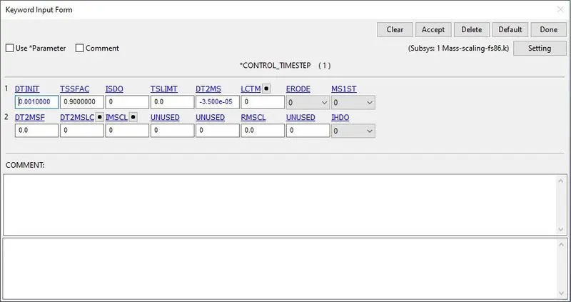
Figure 1: CONTROL_TIMESTEP Card.
In this work, an attempt was given to check the optimum value of the mass scale, by checking the run time.
Objective:
Use mass scaling to find out the optimum value of mass scale for the minimum run time while the %mass error is in the allowable range of 8%.
PROCEDURE
To find out the optimum value of the mass scale, a trial-and-error method was followed. The mass was increased by 10 % in each case, and the runtime and added mass were observed.
Case 1: (No Control Card)
In the first case, the model was run with pre-defined timestep control values. The CONTROL_TIMESTEP card can be seen in fig. 1. The TSSFAC or the timestep scale factor is by default 0.9, and the mass-scale factor of 3.5E-05. The effect of this scale on simulation can be seen in the figure below. In this case, the estimated clock time to complete the simulation was 13 hrs, 25 mins, which is quite a long time for the simulation. There is no detail of mass addition is given, as no such input was provided. Also, the timestep can be seen in the figure below at 4.40E-05.
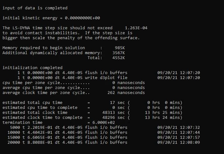
Figure 2: The time information of the first case when no timestep control was used.
Case 2: (DT2MS = -3.5E-05)
In the second case, the model was run with a timestep control card with a dt2ms value of 3.5E-05. The TSSFAC or the timestep scale factor was default 0.9. The effect of this scale on simulation was then observed. In this case, the estimated clock time to complete simulation was increased to 14 hrs, 6 mins, with no added mass (% Added Mass = 0.0%). The details of mass addition can be seen in fig. 3.
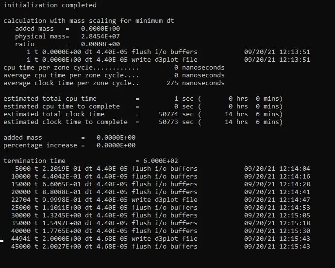
Figure 3: The time information of the second case when the dt2ms was 3.5E-05.
In this case, the information about mass addition can be seen because of the introduction of the dt2ms value. The timestep value hasn’t though changed after inputting the control card.
Case 3: (DT2MS = -5.5E-05)
In the second case, the value of dt2ms in the control card was increased to see the effect on added mass and timestep dt. In the figure below, the estimated clock time to complete simulation was further increased to 15 hrs 49 mins, and the added mass was also increased by 1.3179E-03%. The timestep can be seen decreased from 4.68E-05 (in an earlier case) to 4.50E-05. This is the reason behind the increase in estimated clock time.
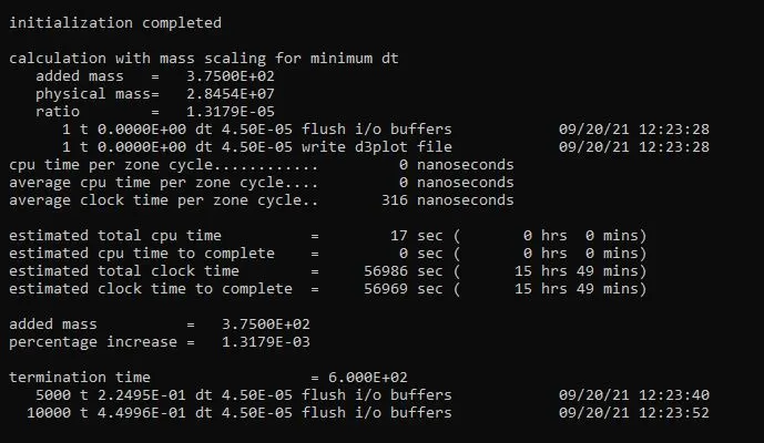
Figure 4: The time information of the second case when the dt2ms was 5.5E-05.
Case 4: (DT2MS = -1.0E-04)
In case 4, the dt2ms value was further increased to -1.0E-04, to investigate the effect. The effect can be seen in the figure below. The artificial mass now can be seen added by 6.423%, which is quite considerable. The timestep has also increased to 9.00E-5. Both of these led to the decrease in the estimated clock time to complete the simulation to 7 hrs 4 mins.
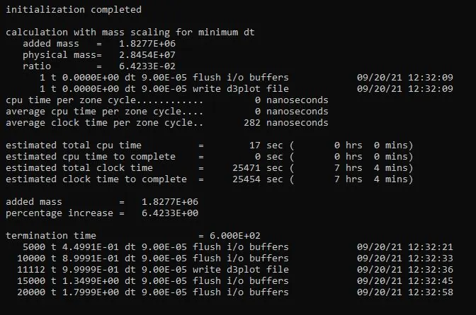
Figure 5: The time information of the fourth case when the dt2ms was 1.0E-04.
Case 5: (DT2MS = -1.0E-04, TSSFAC = 0.7)
In this case, the dt2ms value was kept to -1.0E-04, and the tssfac or timestep scale factor was reduced to 0.7. The effect can be seen in the figure below. The added mass remained the same, as in case 4. Thus, tssfac has not affected the mass addition. However, the dt or the timestep has decreased to 7.00E-05. Also, the estimated clock time to complete was also increased to 9 hrs 44 mins, as timestep was decreased.
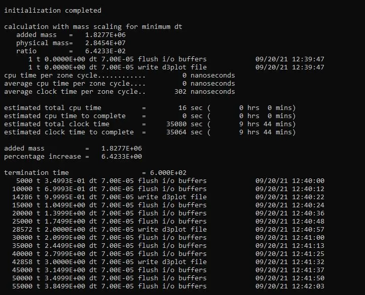
Figure 6: The time information of the fifth case when the dt2ms was 1.0E-04, and the tssfac was 0.7.
Case 6: (DT2MS = -1.5E-04, TSSFAC = 0.8)
In case 6, the dt2mas was increased to 0.8, as it has no effect on added mass, and the mass scale was further increased to -1.5E-04.
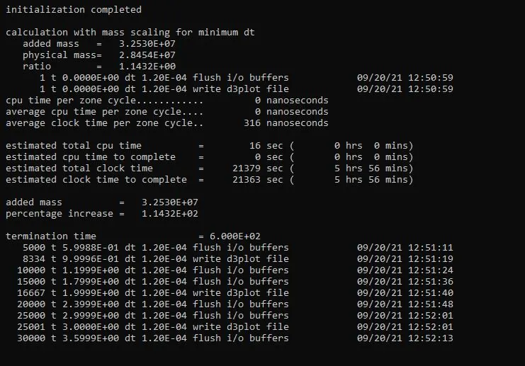
Figure 7: The time information of the sixth case when the dt2ms was increased to -1.5E-04, and the tssfac was 0.8.
In this case, the percent added mass has a significant change of 1.1432E+02, which is not acceptable, as it would have a considerable effect on the inertia. Also, the timestep has also increased remarkably to 1.20E-04.
Case 7: (DT2MS = -1.2E-04, TSSFAC = 0.9)
In case 6, the mass was added too much, thus in this case the dt2ms was decreased slightly to -1.2E-04, and tssfac was kept at a default value of 0.9.
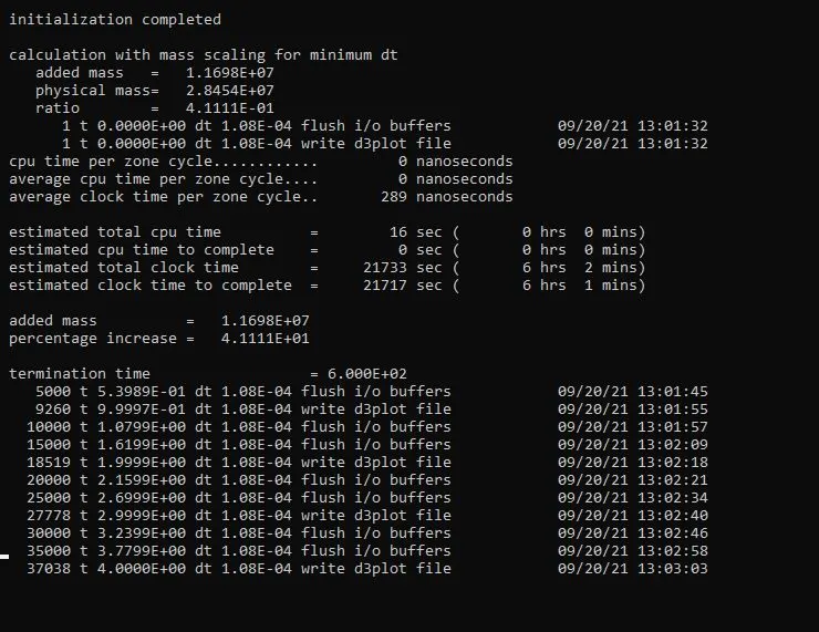
Figure 8: The time information of the seventh case when the dt2ms was decreased to -1.2E-04, and the tssfac were 0.9.
In this case, the percent added mass was decreased, but it is not acceptable, as it is above 8%. Thus, one more case was required to solve.
Case 8: (DT2MS = -1.02E-04, TSSFAC = 0.9)
Case 5 had an acceptable value. Thus, making slight changes to case 5, this case was solved. In this case, the dt2ms value was taken as -1.02E-05 and the tssfac value of 0.9. After initiating the solver, the software showed the estimated clock time to complete of 8 hrs 44 mins, and the added mass was also in the acceptable range of 8%.
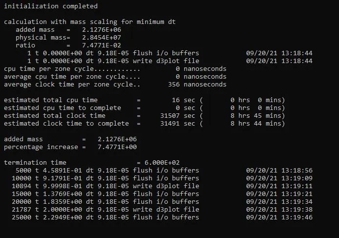
Figure 9: The time information of the eighth case when the dt2ms was decreased to -1.02E-04, and the tssfac was 0.9.
Case 9: (DT2MS = -1.0E-04, TSSFAC = 0.9)
One more attempt was tried in case 9, wherein the dt2ms was kept equal to -1.0E-04 and the timestep scale factor to 0.9.
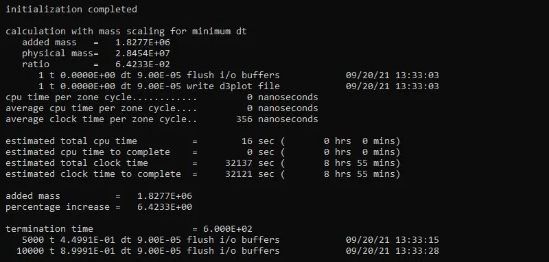
Figure 10: The time information of the ninth case when the dt2ms was decreased to -1.0E-04, and the tssfac were 0.9.
Compared to case 5, in this case, the estimated run time was decreased by around 50 mins, and the artificial mass addition was also in an acceptable range.
The plot shown in fig. 12, shows the collective data of all the cases. In the plot itself, it can be observed that case 4, case 5, case 8, and case 9 performed well. Out of these cases, case 4 is seen to be the optimum combination of dt2ms and tssfac. However, case 4, and case 9 are the same cases (no change). But the change in run-time is due to other system’s programs running in the background. For example, with no other application running in the system, the same case with dt2ms equal to -1.0E-04 and tssfac equal to 0.9 gave the estimated clock time to complete was equal to 5 hrs 13 mins with the mass addition of 6.42%.
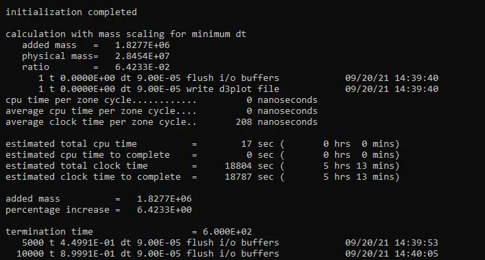
Figure 11: The time information of the case when the dt2ms was -1.0E-04, and the tssfac was 0.9, and no other application running on the system.
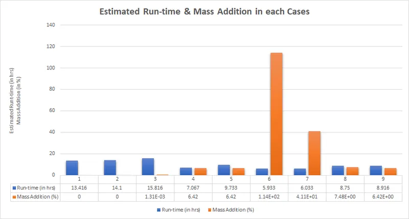
Figure 12: The estimated run-time (in hrs.) and mass addition (in %).
Now, using the data of case 2, and case 4, the same model was run using implicit analysis. Below are the two cases of implicit analysis.
Case 10: (Implicit Analysis: DT2MS = -3.5E-05, & TSSFAC = 0.9)
In this case, there was no clear representation of the estimated time to complete the simulation. However, for the time of 0.1 of the simulation time, it was taking 1 sec. It means for 600s of simulation, it would take approx. 6000 seconds or 100 mins. to solve the problem. Also, there was no mass addition.
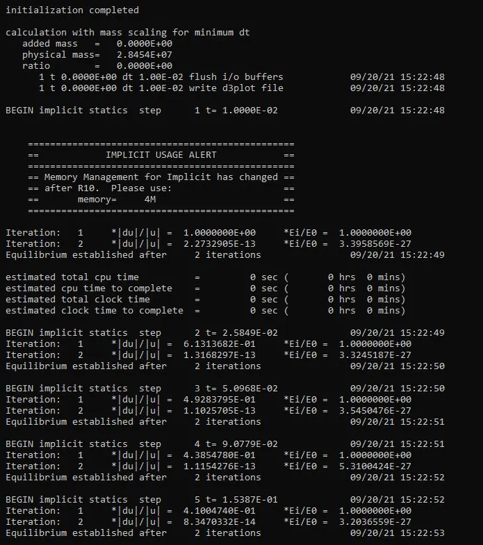
Figure 13: The time information of the implicit analysis case when the dt2ms was -3.5E-05, and the tssfac was 0.9.
Case 11: (Implicit Analysis: DT2MS = -1.0E-04, & TSSFAC = 0.9)
In this case, the optimum value of dt2ms and tssfac was taken equal to -1.0E-04, and 0.9 respectively. In the figure below it can be seen that the added mass was 0.0%, even after increasing the dt2ms. Also, the time the simulation would take for solving the problem is also same equal to 100 mins. It clearly shows that how explicit analysis is conditionally stable, and implicit analysis is not.
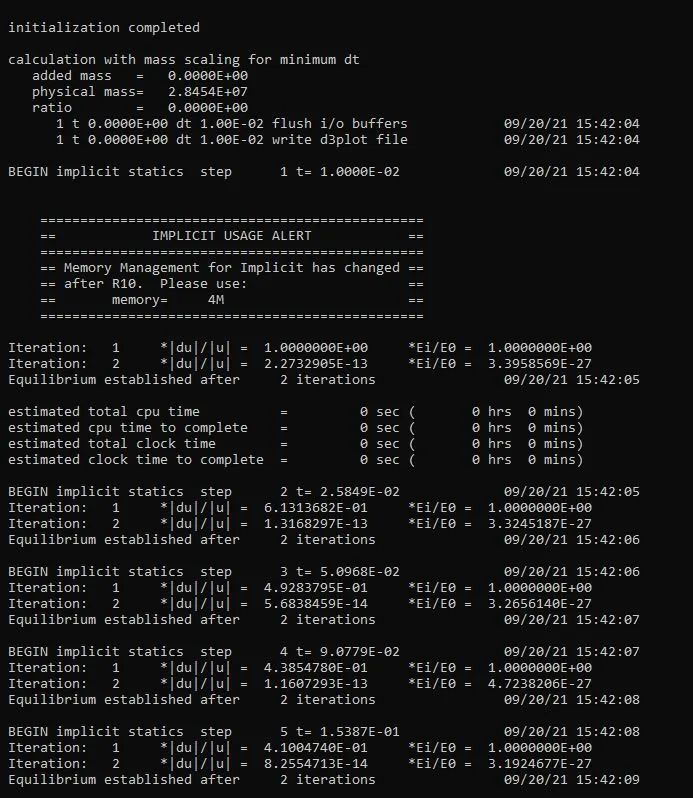
Figure 13: The time information of the implicit analysis case when the dt2ms was -1.0E-04, and the tssfac was 0.9.
CONCLUSION:
The simulation was solved to find out the optimum value of the dt2ms and tssfac, and their effect on the runtime. After solving 9 cases, it was observed that case 4 had an optimum value of dt2ms = -1.0E-04, and the tssfac value equal to 0.9. In that case, the estimated runtime was 7 hrs 4 mins. The simulation was solved using implicit analysis for two cases. In the first case, dt2ms value was -3.5E-05, and tssfac was 0.9, and in the second case, dt2ms was -1.0E-04, and tssfac was 0.9. In both cases, no mass addition was there, and the simulation time was also the same. It clearly shows that how explicit analysis is conditionally stable, and implicit analysis is not.
References:
[1] https://www.dynasupport.com/howtos/general/mass-scaling