Week - 8 Mass Scaling
AIM OF THE PROJECT
- Reduce the runtime required to run the analysis of a given problem by mass scaling and ensure the stability of mass scaling.
- Optimization of DT and TSSFAC parameters.
- The hard limit on mass scaling is 8%
- Plot a Histogram for comparing runtime with mass scaling results.
- Run the given model using implicit solver with necessary changes.
- Comparing the implicit and explicit runtime.
INTRODUCTION TO MASS SCALING
Mass scaling is one of the methods used in many industries to reduce the runtime of a finite element analysis. It is also referred as a technique where a non physical mass is added to the simulation in order to increase the timestep size and thereby using less runtime.
*CONTROL_TIMESTEP will set the structural timestep size control using different options. Some of the variables in the card used for mass scaling are TSSFAC and DT2MS. Mass scaling can be done by altering the values of these variables.
- DT2MS is used to define new timestep required for the simulation and thus affects additional mass provided for the simulation
- TSSFAC does not affect the mass scaling, but it will affect the timestep size and the simulation speed. Timestep is defined as a product of TSSFAC and DT2MS.
INTRODUCTION TO TIME STEP
In the context of Finite Element Analysis, time step is the time required for a shock wave to propogate across the smallest distance of the element.
- The time step is calculated by using this formula, ΔT = L / C
- C = sqrt(E/ρ)
- ΔT = Scaling factor, L = Smallest length of the element
- E = Young's modulus of a material, ρ = density of a material
GIVEN MODEL
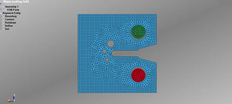
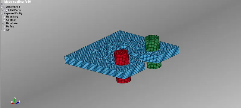
PROCEDURE TO BE FOLLOWED FOR PERFROMING EXPLICIT ANALYSIS
Explicit analysis on the given model can be performed in two ways. Performing the simulation without mass scaling is the first type and performing the simulation with mass scaling is the second type.
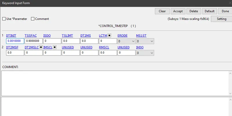
Type 1: Performing the simulation without mass scaling. It means DT2MS should be zero and end time of the simulation should be given as 600 ms
i)Specify the value of DT2MS as zero in *CONTROL_TIMESTEP
(ii) Save the model using .k extension and run the simulation using LS-Run
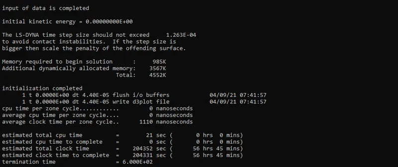
CONCLUSION: The estimated simulated time without mass scaling is 56 hours and 45 minutes. To reduce the clock time, mass should be added to the elements which inturn increases the speed of time step.
Type 2: Performing the simulation with mass scaling.
Step 1: Load the values of TSSFAC as 0.9 and D2TMS values should be kept varying.
i)Specify the value of TSSFAC as 0.9 and D2TMS as -3.5e-05 in *CONTROL_TIMESTEP
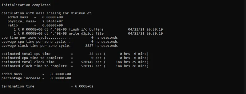
ii)Specify the value of TSSFAC as 0.9 and D2TMS as -5e-05 in *CONTROL_TIMESTEP
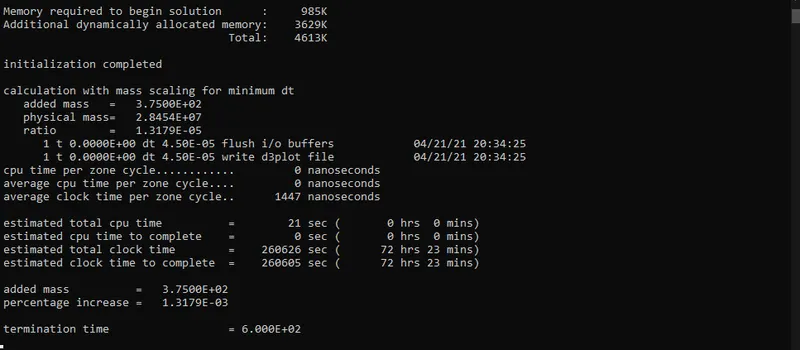
iii)Specify the value of TSSFAC as 0.9 and D2TMS as -7e-05 in *CONTROL_TIMESTEP
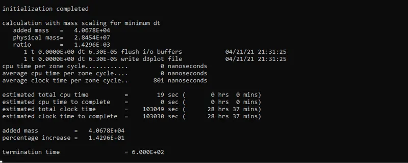
iv)Specify the value of TSSFAC as 0.9 and D2TMS as -9e-05 in *CONTROL_TIMESTEP
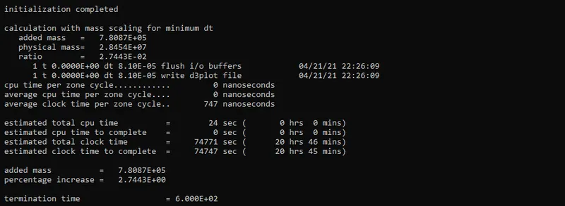
v)Specify the value of TSSFAC as 0.9 and D2TMS as -1e-04 in *CONTROL_TIMESTEP
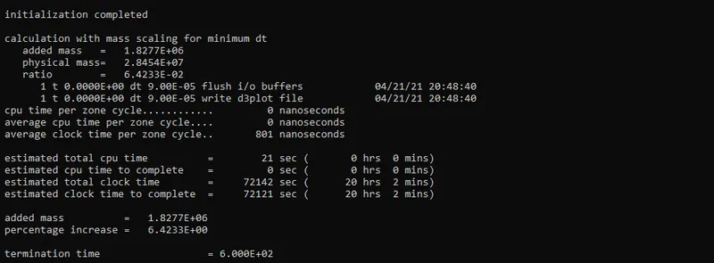
vi)Specify the value of TSSFAC as 0.9 and D2TMS as -1.03e-04 in *CONTROL_TIMESTEP
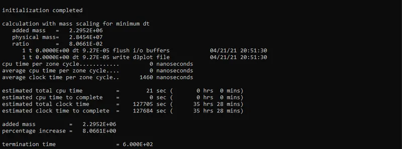
vii) Since there is a slight increase in percentage increase when D2TMS is specified as -1.03e-04, so change the value of -1.028e-04. TSSFAC will be 0.9
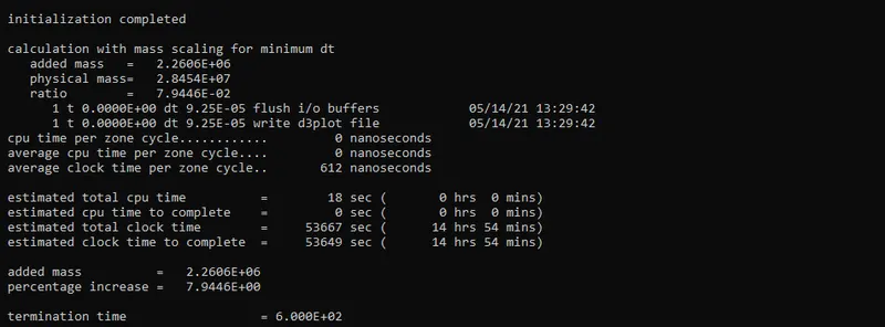
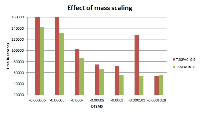
The following tabe shows the results for different cases of explicit analysis with TSSFAC as 0.9
| DT2MS | Mass added | % Mass added | Total time(Hours and Mins) | Total time(seconds) |
| -0.0000350 | 0 | 0 | 144 hrs 29 mins | 520145 |
| -0.0000500 | 375 | 0.0013179 | 72 hrs 23 mins | 260626 |
| -0.0000700 | 40670 | 0.14296 | 28 hrs 37 mins | 103049 |
| -0.0000900 | 780870 | 2.7443 | 20 hrs 45 mins | 74771 |
| -0.0001000 | 1827700 | 6.4233 | 20 hrs 2 mins | 72142 |
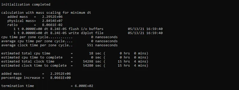
| -0.0001030 | 2295200 | 8.0661 | 21 hrs 34 mins | 127705 |
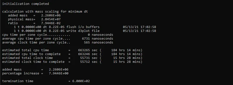
| -0.0001028 | 2260600 | 7.9446 | 14 hrs 54 mins | 53667 |
Step 2: Load the values of TSSFAC as 0.8 and D2TMS values should be kept varying.
i)Specify the value of TSSFAC as 0.8 and D2TMS as -3.5e-05 in *CONTROL_TIMESTEP
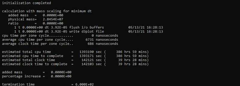
ii)Specify the value of TSSFAC as 0.8 and D2TMS as -5e-05 in *CONTROL_TIMESTEP
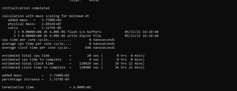
iii)Specify the value of TSSFAC as 0.8 and D2TMS as -7e-05 in *CONTROL_TIMESTEP
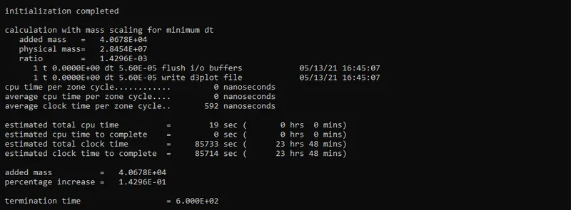
iv)Specify the value of TSSFAC as 0.8 and D2TMS as -9e-05 in *CONTROL_TIMESTEP
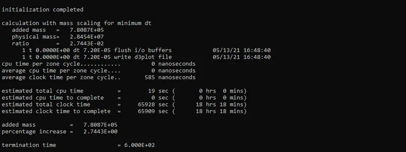
v)Specify the value of TSSFAC as 0.8 and D2TMS as -1e-04 in *CONTROL_TIMESTEP
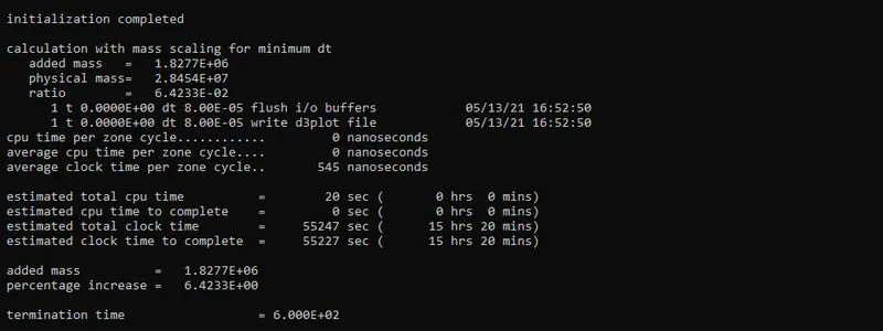
vi)Specify the value of TSSFAC as 0.8 and D2TMS as -1.03e-04 in *CONTROL_TIMESTEP
vi)Specify the value of TSSFAC as 0.8 and D2TMS as -1.028e-04 in *CONTROL_TIMESTEP
The following tabe shows the results for different cases of explicit analysis with TSSFAC as 0.8
| DT2MS | Mass added | % Mass added | Total time(Hours and Mins) | Total time(seconds) |
| -0.0000350 | 0 | 0 | 39 hrs 28 mins | 142121 |
| -0.0000500 | 375 | 0.0013179 | 36 hrs 22 mins | 130929 |
| -0.0000700 | 40678 | 0.14296 | 23 hrs 48 mins | 85733 |
| -0.0000900 | 780870 | 2.7443 | 18 hrs 18 mins | 65928 |
| -0.0001000 | 1827700 | 6.4233 | 15 hrs 20 mins | 55247 |
| -0.0001030 | 2295200 | 8.0661 | 15 hrs 04 mins | 54298 |
| -0.0001028 | 2260600 | 7.9446 | 15 hrs 28 mins | 55731 |
PROCEDURE TO BE FOLLOWED FOR PERFROMING IMPLICIT ANALYSIS
The given model should be made to run with the help of Implicit analysis and the run time of Implicit analysis and the run time of explicit analysis should compared. The following cards are to be used in order to perform Implicit analysis for the given model.
Step 1: Define control cards required to run implicit analysis
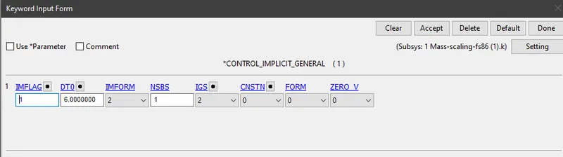
(i) *CONTROL_IMPLICIT_GENERAL:- This card should be used when the problem is to be shifted from Explicit analysis to Implicit analysis. IMFLAG should be loaded as 1 in order to activate Implicit analysis. IMFORM should be loaded as 2 because it can retain back to original element formulation
IMFLAG - Implicit/Explicit switching flag
DTO - Initial time step size for implicit analysis
IMFORM - Element formulation switching
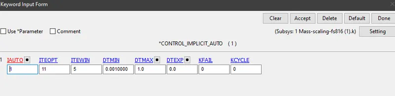
(ii) *CONTROL_IMPLICIT_AUTO:- This card will define parameters for automatic time step control during Implicit analysis. IAUTO should be loaded as 1 in order to adjust the time step automatically.
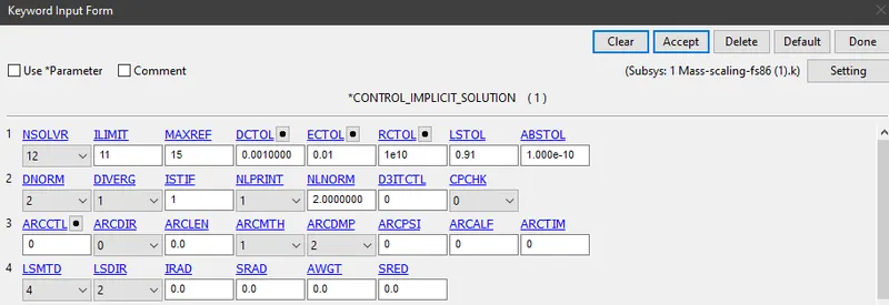
(iii) *CONTROL_IMPLICIT_SOLUTION: This card is used to apply implicit calculations. Use of this card is used to specify whether a linear or nonlinear solution is desired.
NSOLVR - Solution method for implicit analysis (The value is 12, as it is a Non-Linear problem)
ILIMIT - Iteration limit between automatic stiffness reformations. By default the value will be 11
MAXREF - Stiffness reformation limit per time step. The value is given as 15
DCTOL - Displacement relative convergence tolerance. The value is given as 0.001
DNORM - Displacement norm for convergence test. The value is given as 2
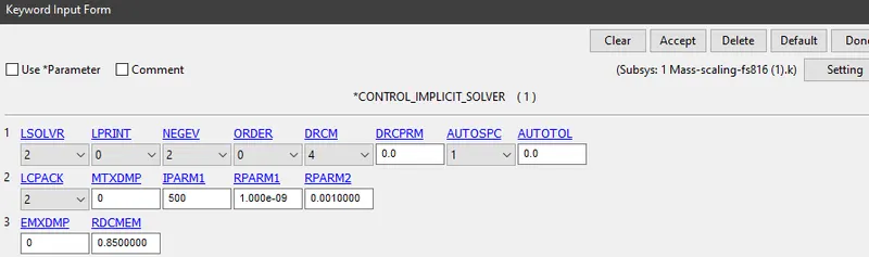
(iv) *CONTROL_IMPLICIT_SOLVER: This card is used to apply implicit calculations. The linear equation solver performs the CPU-intensive stiffness matrix inversion.
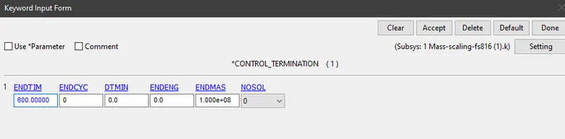
(v) *CONTROL_TERMINATION: The end time of the simulation is given as 600 ms
Step 2: DT2MS=-3.5e-5 is given with TSSFAC=0.9
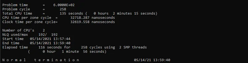
Step 3: DT2MS=-1e-4 is given with TSSFAC=0.9
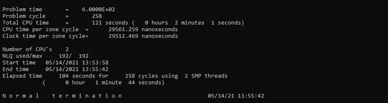
Step 4: DT2MS=-1.028e-4 is given with TSSFAC=0.9

Important points to be noted
- From the above three cases it is clear that for a TSSFAC value of 0.9 with varied DT2MS. DT2MS and TSSFAC do not affect simulation time as the implicit analysis do not use a physical time factor.
- Initial time step DTO = Termination time / 100 = 600/100 = 6
- Initial time step is defined in *CONTROL_IMPLICIT_GENERAL
- The simulation time and time step is mainly controlled using *CONTROL_IMPLICIT_AUTO with parameters such as ITEOPT, ITEWIN, DTMIN and DTMAX
FINAL CONCLUSION
- Mass scaling is achieved by varying the values of DT2MS and TSSFAC for a given model using trial and error method
- Mass scaling is useful only for explicit analysis where the difference in simulation time is too large
- Percentage of increase in mass is not reported in implicit analysis
- Mass scaling does not affect simulation time in case of implicit analysis
- Learned the concept of mass scaling and its availability in explicit analysis