Week - 2 - Explicit and Implicit Analysis

EXPLICIT AND IMPLICIT METHODS

Aim: To solve the equation F(u) = u³ + 9u² + 4u using both explicit analysis and implicit analysis methods. Here incremental load control scheme is used

DETAILED EXPLANATION ABOUT EXPLICIT AND IMPLICIT METHODS

Implicit and explicit methods are two types of approaches that can be used to solve finite element problem. The implicit approach is useful in problems in which time dependency of the solution is not an important factor(Static structutal, harmonic and model analysis) whereas explicit method is most helpful in solving time dependent problems such as crash, blast, impact and so on

Explicit method: Explicit analysis aim to solve for acceleration (or otherwise {x´´}). In explicit analysis for each increment we have to update stiffness matrix, next increment of load defined and the solution is obtained directly. Here we can use Central difference methods. This method is computationally efficient for large models with relatively short dynamic response time and it depends on wave propagation speed, characterstic length of an element Explicit method handles non linearities with relative ease as compared to implicit analysis. It is used when velocity/strain rates is greater than 10 units/sec.

Explicit method is a good choice for wave propogation type of problems such as car crash, drop test, Impact, Blast and so on

If the nonlinear force versus displacement is relationship is not known, but the stiffness is known, it is possible to construct the graph of force versus displacement numerically. Here Incremental explicit load control scheme is used.

So the given equation is, Force= F(u) = u³ + 9u² + 4u

Differentiating force with respect to displacement

Stiffness = K(u) = = 3u² + 18u + 4

Here three equal load increments of ∆F = 1 unit are used to load the tension bar.

The variables used are u for displacement, f for internal force in the bar, F for external force applied to the bar and k for stiffness. Incremental displacements or incremental externally applied forces are represented as ∆u or ∆F.

The relation used to find the incremental displacement, ∆F = k (∆u)

u = Displacement, f = Internal force in the bar, F = External force in the bar

∆u = Incremental displacements, ∆F = Incremental external applied force

Step 1:

u₀ = 0, ∆F = 1

k(u₀) = 3(0) + 18(0) + 4 = 4

∆u₁ = ∆F/k(u₀) = 1/4 = 0.25

u₁ = u₀ + ∆u₁ =0 + 0.25 = 0.25

F_ext = ∆F = 1

f_int = u³ + 9u² + 4u = (0.25)³ + 9(0.25)² + 4(0.25) = 1.5781 (Here u = u₁)

Step 2:

u₁ = 0.25

k(u₁) = 3(0.25)² + 18(0.25) + 4 = 8.6875

∆u₂ = ∆F/k(u₁) = 1/8.6875 = 0.1151

u₂ = u₁ + ∆u₂ = 0.25 + 0.1151 = 0.3651

F_ext = ∆F + ∆F = 2

f_int = u³ + 9u² + 4u = (0.3651)³ + 9(0.3651)² + 4(0.3651) = 2.708 (Here u = u₂)

Step 3:

u₂ = 0.3651

k(u₂) = 3(0.3651)² + 18(0.3651) + 4 = 10.9717

∆u₃ = ∆F/k(u₂) = 1/10.9717 = 0.09114

u₃ = u₂ + ∆u₃ = 0.3651 + 0.09114 = 0.4562

F_ext = ∆F + ∆F + ∆F = 1+1+1=3

f_int = u³ + 9u² + 4u = (0.4562)³ + 9(0.4562)² + 4(0.4562) = 3.7915 (Here u = u₃)

It is evident from the results that external forces and internal forces are not in equilibrium because F_ext ≠ f_int

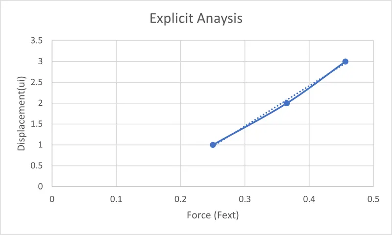
The results of explicit analysis are as shown in the form of table

Step	∆Fi	∆ui	ui	(Fext)i	(fint)i	Range fint - Fext
1	1	0.25	0.25	1	1.5781	0.5781
2	1	0.1151	0.3651	2	2.708	0.708
3	1	0.09114	0.4562	3	3.7915	0.7915

Graph: A plot of displacement versus force as shown below for explicit method

Implicit method: In implicit analysis for each increment we have to update stiffness matrix, next increment of load defined and the solution is obtained by Newton-Raphson method. Here we can use various methods Beta-Newmark method of second order and Euler method of first order. This method is extremely time consuming for large models with no mathematical time limit for solution. It is used when velocity/strain rates is lower than 10 units/sec

Implicit method is a good choice for structural dynamic problems for which load rate is low.

An implicit analysis is same as the explicit analysis, except that at the end of each step Newton-Raphson iterations are used to enforce equilibrium before moving to next step. Internal forces and external forces will not be in equilibrium unless the stiffness is linear for the given step. Hence in order to achieve equilibrium corrections must be made to the displacement.

To minimise the residual, R = F_internal - F_external

Expanding the residual as a Taylor series about the current displacement u^j gives

R ^j+1 = R^j (u^j) + dR(uj)/du . δu ^j+1 + ……… = R^j + k(u^j) δu ^j+1 + ……………

By neglecting higher order terms in the series, setting R ^j+1 = 0 and solving for δu ^j+1 the following correction is obtained.

The implicit analysis proceeds as follows

Step 1:

u₀ = 0, ∆F = 1

k(u₀) = 3(0) + 18(0) + 4 = 4

∆u₁ = ∆F/k(u₀) = 1/4 = 0.25

u₁ = u₀ + ∆u₁ =0 + 0.25 = 0.25

Checking the residual,

F_ext = ∆F = 1

F_int = u³ + 9u² + 4u = (0.25)³ + 9(0.25)² + 4(0.25) = 1.5781 (Here u = u₁)

R⁽⁰⁾ = F_internal - F_external = 1.5781 – 1 = 0.5781

R⁽⁰⁾ > 10^-2 (Newton-Raphson iterations are necessary)

Calculate the correction to u₁ = u₁⁽⁰⁾

δu¹ = -[k (u₁⁽⁰⁾)]^-1 . R⁽⁰⁾ = -(8.6875)^-1 x 0.578 = -0.0665

The updated value of u₁⁽¹⁾ = u₁⁽⁰⁾ + δu¹ = 0.25 – 0.0665 = 0.1835

Checking the residual again,

F_ext = ∆F = 1

F_int = (u₁⁽¹⁾)³ + 9(u₁⁽¹⁾)² + 4 u₁⁽¹⁾ = 0.1835³ + 9(0.1835)² + 4(0.1835) = 1.0432

R⁽¹⁾ = F_internal - F_external = 1.0432 – 1 = 0.0432

R⁽¹⁾ > 10^-2 (Newton-Raphson iterations are necessary)

Calculate the correction to u₁ = u₁⁽⁰⁾

δu⁽²⁾ = δu⁽¹⁾ - [k (u₁⁽¹⁾)]^-1 . R₀ = -0.0665 – (7.404)^-1 x 0.0432 = -0.0723

The updated value of u₁⁽²⁾ = u₁⁽⁰⁾ + δu¹ = 0.25 – 0.0723 = 0.1777

F_ext = ∆F = 1

F_int = (u₁⁽²⁾)³ + 9(u₁⁽²⁾)² + 4 u₁⁽²⁾ = 0.1777³ + 9(0.1777)² + 4(0.1777) = 1.0006

R⁽²⁾ = F_internal - F_external = 1.0006 – 1 = 0.0006

R⁽²⁾ > 10^-2 (Newton-Raphson iterations are not necessary)

Therefore the final value is u₁ = u₁⁽²⁾ = 0.1777

Step 2:

u₁ = 0.1777, ∆F = 1

k(u₁) = 3(0.1777)² + 18(0.1777) + 4 = 7.2933

∆u₂ = ∆F/k(u₁) = 1/7.2933 = 0.1371

u₂ = u₁ + ∆u₂ =0.1777 + 0.1371 = 0.3148

Checking the residual,

F_ext = ∆F + ∆F = 2

F_int = u³ + 9u² + 4u = (0.3148)³ + 9(0.3148)² + 4(0.3148) = 2.1822 (Here u = u₂)

R⁽⁰⁾ = F_internal - F_external = 2.1822 – 1 = 0.1822

R⁽⁰⁾ > 10^-2 (Newton-Raphson iterations are necessary)

Calculate the correction to u₁ = u₁⁽⁰⁾

δu¹ = -[k (u₂⁽⁰⁾)]^-1 . R⁽⁰⁾ = -(9.9637)^-1 x 0.1822 = -0.0182

The updated value of u₂⁽¹⁾ = u₂⁽⁰⁾ + δu¹ = 0.3148 – 0.0182 = 0.2966

Checking the residual again,

F_ext = ∆F + ∆F = 2

F_int = (u₂⁽¹⁾)³ + 9(u₂⁽¹⁾)² + 4 u₂⁽¹⁾ = 0.2966³ + 9(0.2966)² + 4(0.2966) = 2.0042

R⁽¹⁾ = F_internal - F_external = 2.0042 – 2 = 0.0042

R⁽¹⁾ < 10^-2 (Newton-Raphson iterations are not necessary)

Therefore the final value is u₂ = u₂⁽¹⁾ = 0.2966

Step 3:

u₂ = 0.2966, ∆F = 1

k(u₂) = 3(0.2966)² + 18(0.2966) + 4 = 9.6027

∆u₃ = ∆F/k(u₂) = 1/9.6027 = 0.1041

u₃ = u₂ + ∆u₃ =0.2966 + 0.1041 = 0.4007

Checking the residual,

F_ext = ∆F + ∆F + ∆F = 1 + 1 + 1 = 3

F_int = u³ + 9u² + 4u = (0.4007)³ + 9(0.4007)² + 4(0.4007) = 3.1121 (Here u = u₃)

R⁽⁰⁾ = F_internal - F_external = 3.1121 – 3 = 0.1121

R⁽⁰⁾ > 10^-2 (Newton-Raphson iterations are necessary)

Calculate the correction to u₂ = u₂⁽⁰⁾

δu² = -[k (u₃⁽⁰⁾)]^-1 . R⁽⁰⁾ = -(11.6942)^-1 x 0.1121 = -0.00958

The updated value of u₃⁽¹⁾ = u₃⁽⁰⁾ + δu² = 0.4007 – 0.00958 = 0.3911

Checking the residual again,

F_ext = ∆F + ∆F + ∆F = 1 + 1 + 1 = 3

F_int = (u₃⁽¹⁾)³ + 9(u₃⁽¹⁾)² + 4 u₃⁽¹⁾ = 0.3911³ + 9(0.3911)² + 4(0.3911) = 3.0008

R⁽¹⁾ = F_internal - F_external = 3.0008 – 3 = 0.0008

R⁽¹⁾ < 10^-2 (Newton-Raphson iterations are not necessary)

Therefore the final value is u₃ = u₃⁽¹⁾ = 0.3911

The results of implicit analysis are as shown in the form of table

Step	∆Fi	ui	(Fext)i	(Fint)i	Residual Fint - Fext
1	1	0.1777	1	1.0006	0.0006
2	1	0.2966	2	2.0042	0.0042
3	1	0.3911	3	3.0008	0.0008

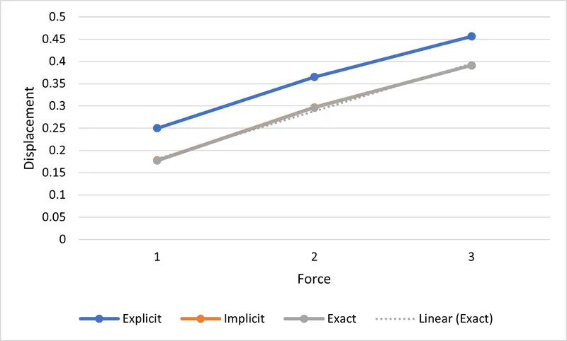
Graph: Comparison between Implicit, Explicit and Exact

Result:

1. Thus, a non linear analysis is shown using incremental explicit and implicit procedure. The results are plotted for comparision
2. As shown in the graph, explicit solution drifts from the exact solution.
3. Implicit method is more accurate than explicit method but the time consumption is more in implicit method.