Week - 8 Mass Scaling

• Aim-
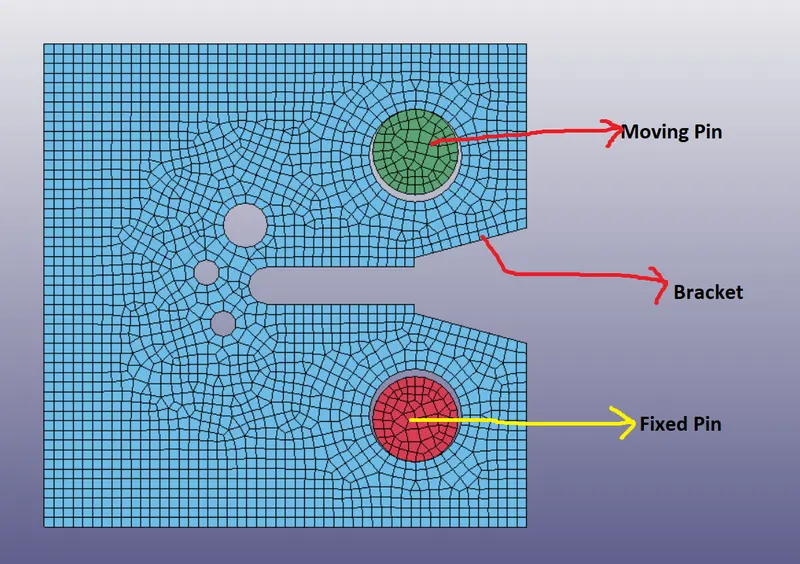
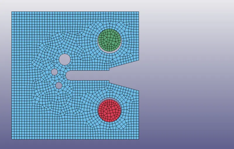
  • The aim of this challenge is to compare the time taken by explicit and implicit ways of solving for below problem.
    • 
• Procedure-
  1. The first step is to open the given in a new LS-Prepost window.
     • 
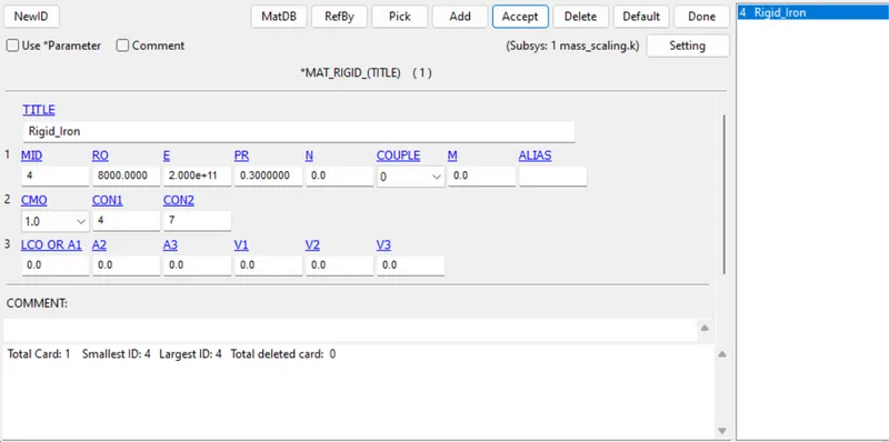
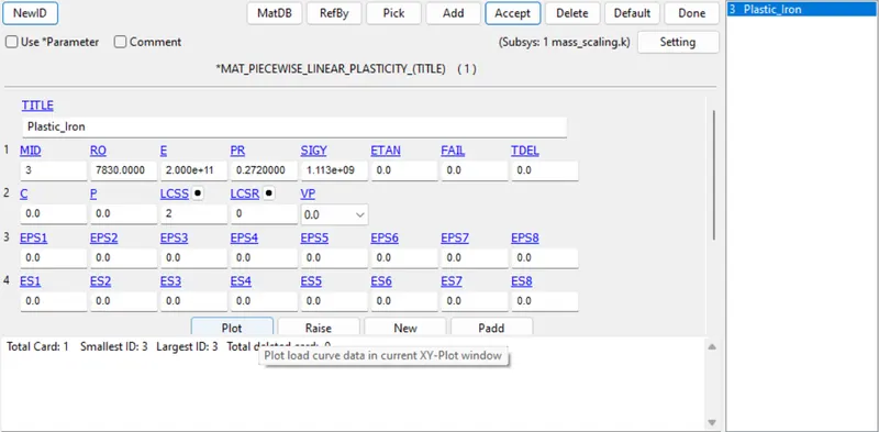
  2. As the section ID is defined earlier now we move to the next step which is defining material ID. Here we've to define two materials rigid and piecewise linear plasticity formulated. The rigid material type is for the pins and the piecewise linear plasticity one is for the plate. Both material cards are given below
     • Rigid material card-
       
       • 
     • Piecewise linear plasticity material card-
       • 
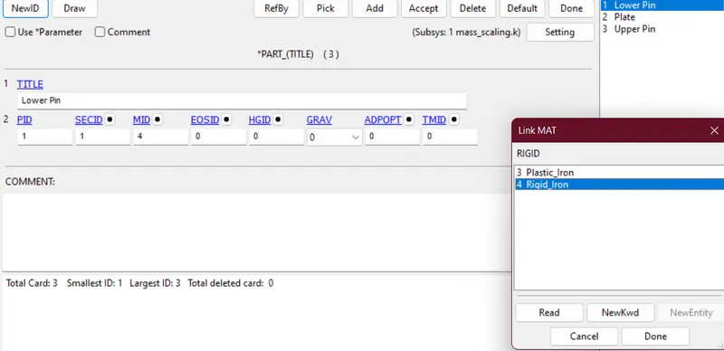
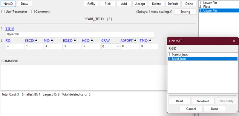
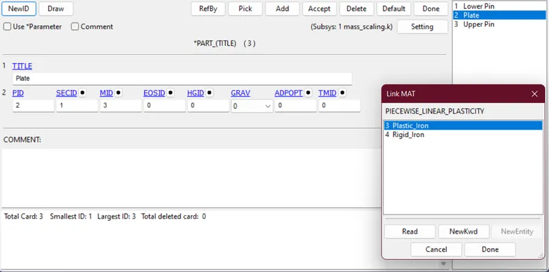
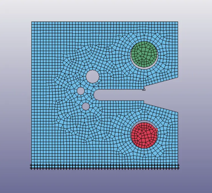
  3. The next step is to check the part ID and check the names of each part are correct or not. In our case the upper pin(PID 1) is green, the lower pin(PID 3) is red in colour and the plate(PID 2) is blue in colour. Now we assign the material property to each part and update the part card.
     • Lower pin part card-
       • 
     • Upper pin part card-
       • 
     • Plate part card-
       • 
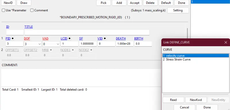
  4. The next step is to apply boundary conditions to the plate and pin. First, we fix the plate and lower pin using the Boundary_SPC. Then we give Boundary_Prescribed_motion to the upper pin to see how the plate reacts to the motion.
     • Spc-
       • 
     • Prescribed motion-
       • 
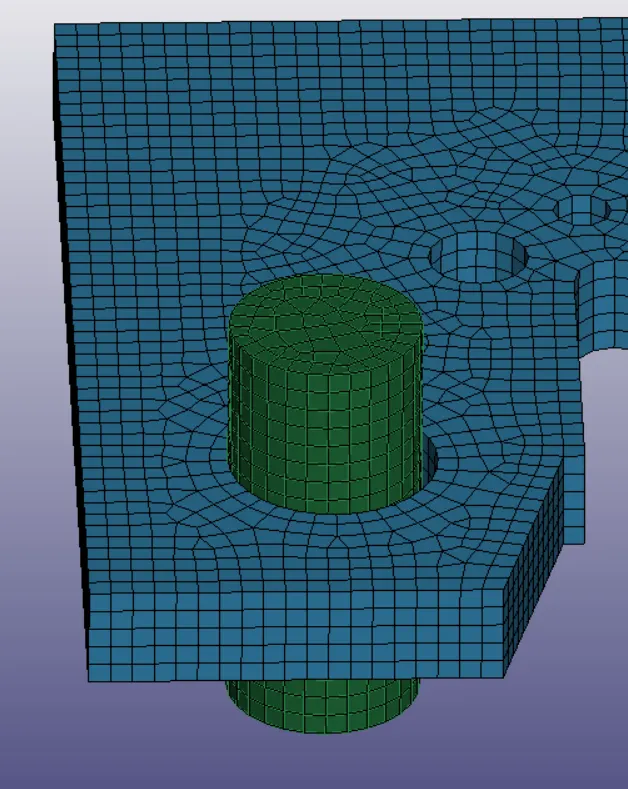
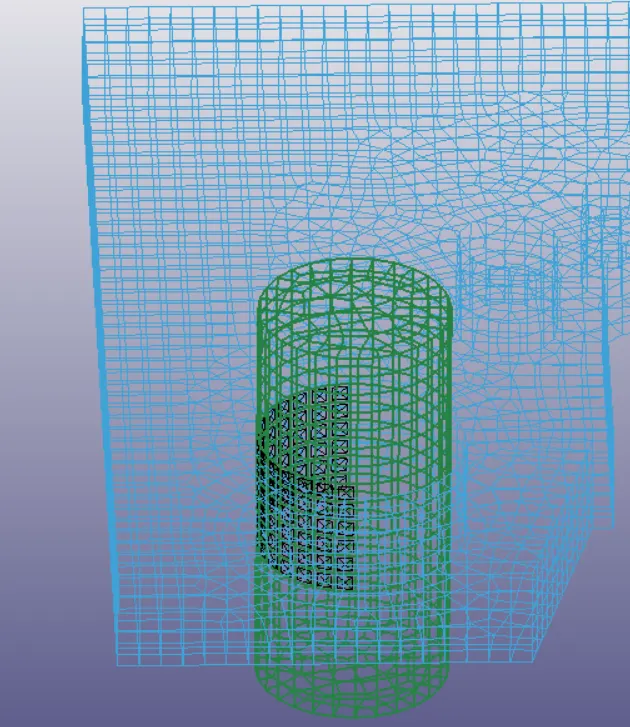
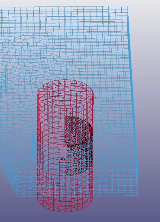
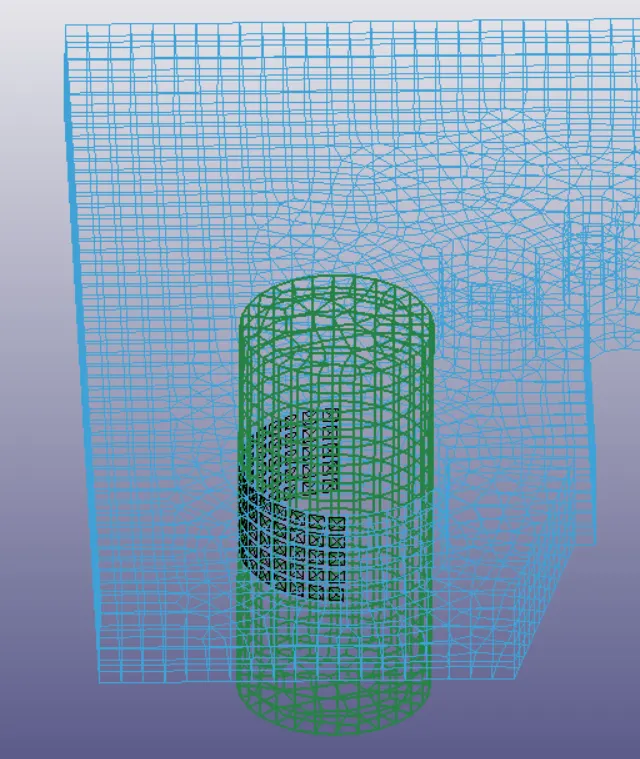
  5. The next step is to create different segments in order to define contact properly. Here we've created four segments
     • Upper pin contact
       • 
     • Lower pin contact
       • 
     • Upper hole contact
       • 
     • Lower hole contact
       • 
  6. All the above data will remain the same for both implicit and explicit analysis.

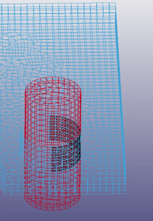
How do explicit and implicit compares?

In simple words, explicit analysis is used for fast analysis and implicit analysis is used for slow analysis. An explicit analysis involves a very straightforward small time step increment and the effect of acceleration is considered while solving the solver doesn't try to converge with each timestep. While Implicit shares some similarities with explicit analysis but it iteratively tries to converge after each time step this effectively gives implicit a flexibility to solve with large time steps but it takes a lot of computational time to find the proper equilibrium.

1. Explicit analysis
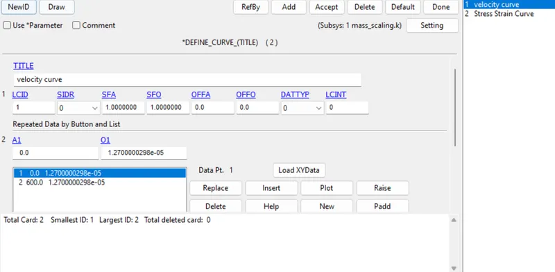
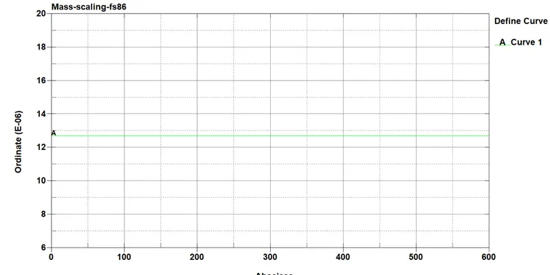
   1. In the case of explicit, we provide motion as velocity to the upper pin by defining a constant velocity curve.
      1. The velocity curve is given below-
         • 
         • 
      2. Defining velocity curve to the Boundary_Prescribed_Motion-
         • 
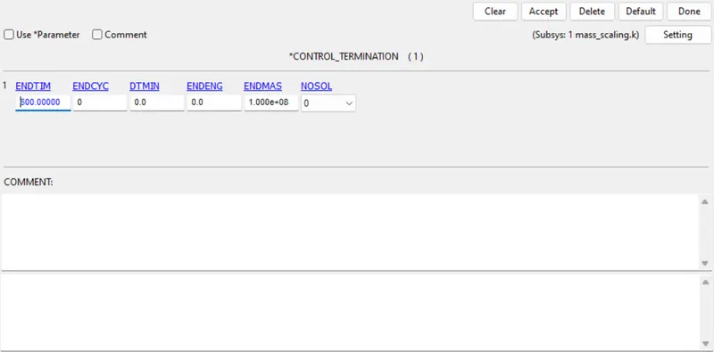
   2. The next step is to give the control cards such as termination and timestep cards.
      1. As the unit system is in kg-m-s we have to consider a greater termination time here it is 600s.
         • 
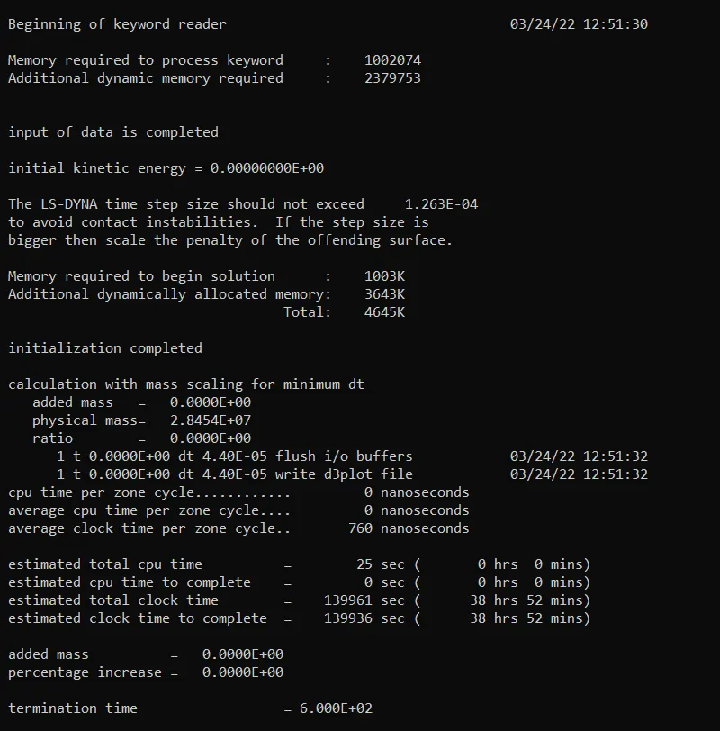
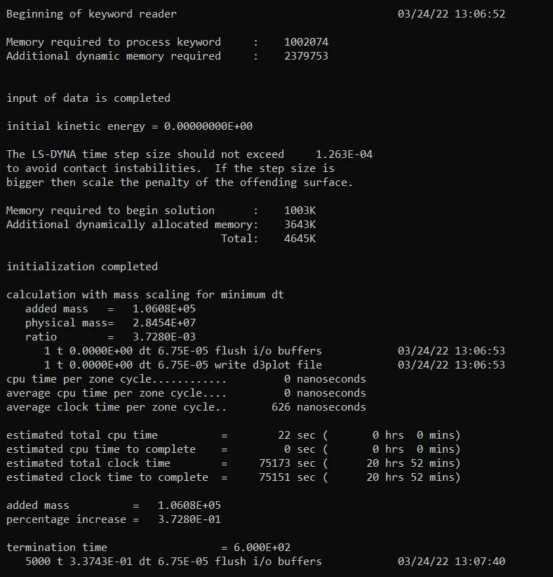
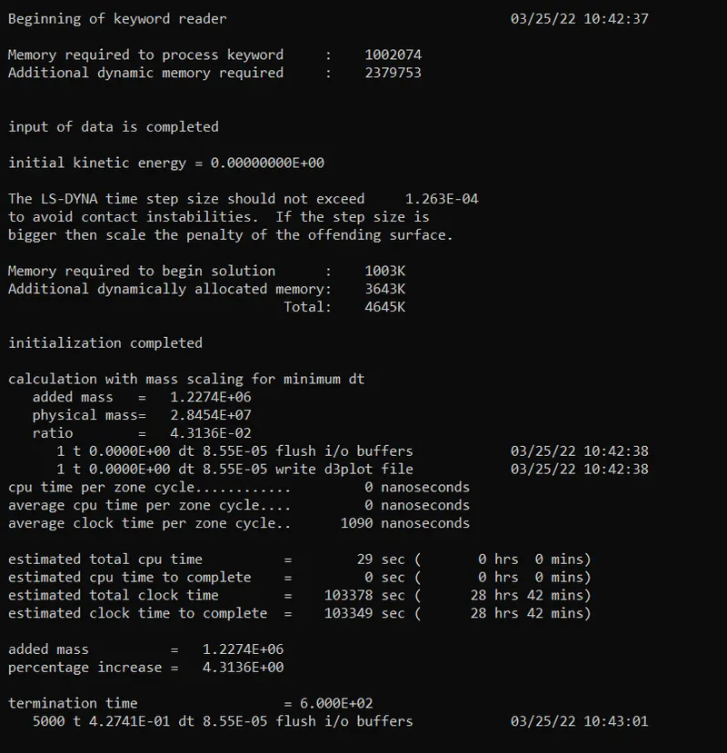
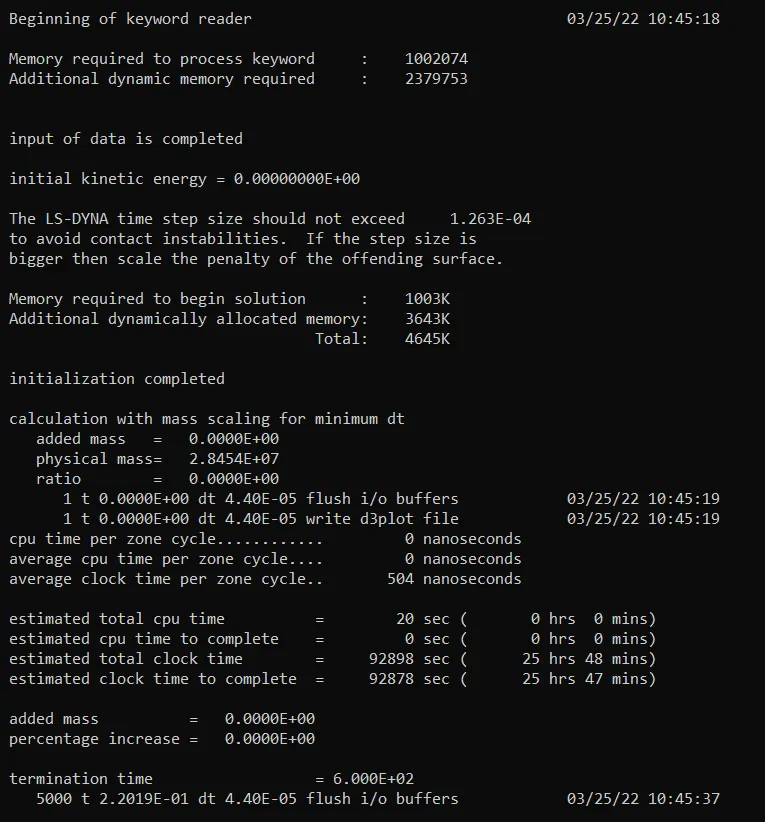
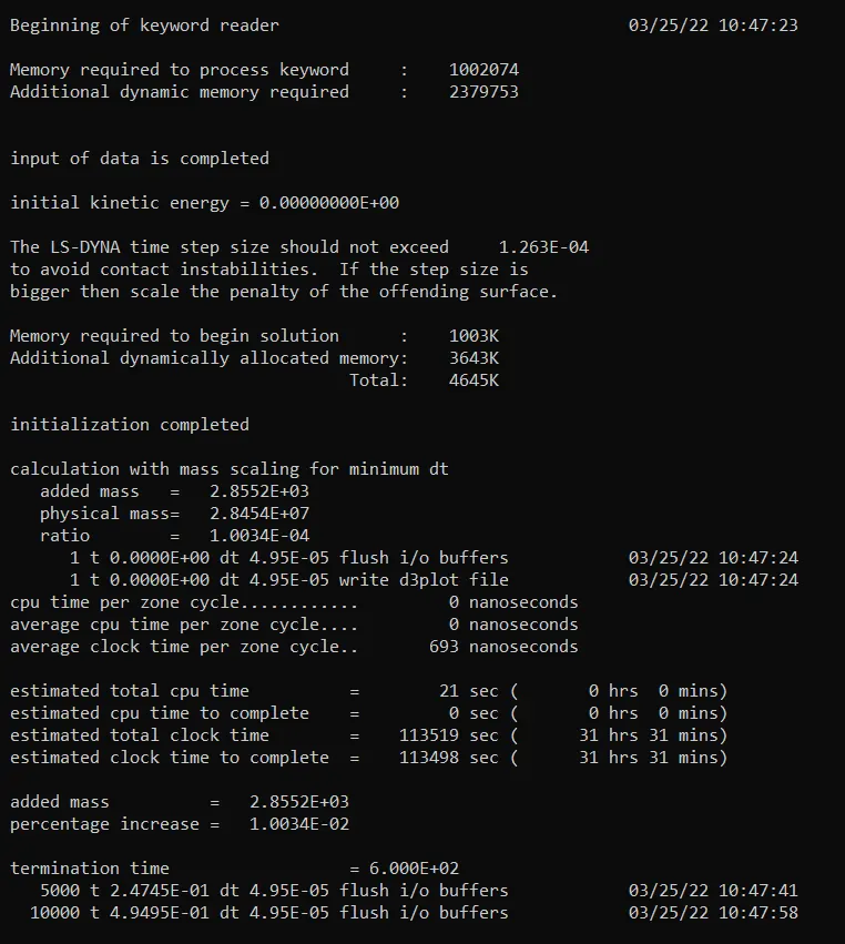
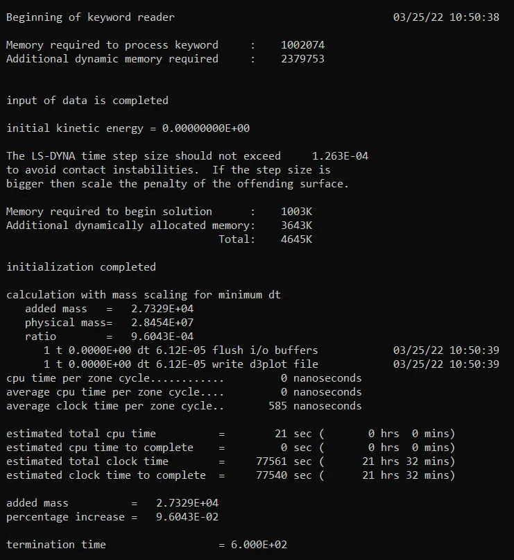
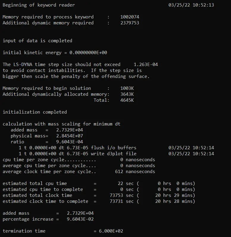
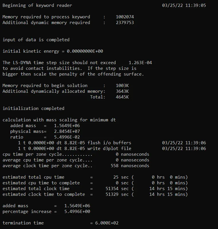
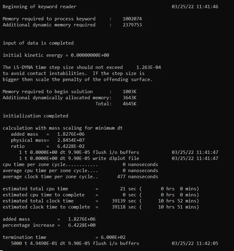
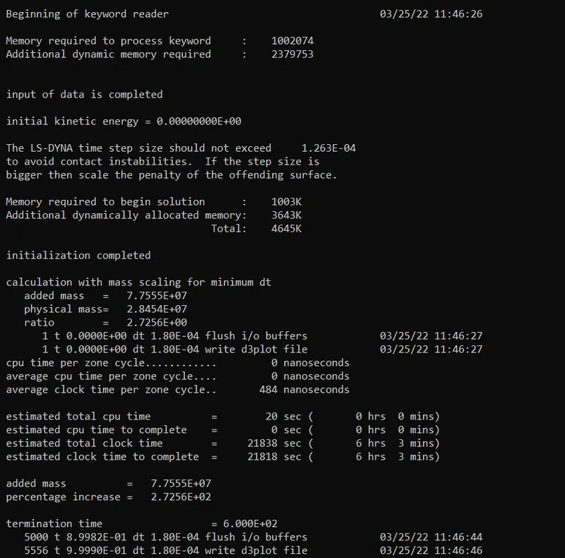
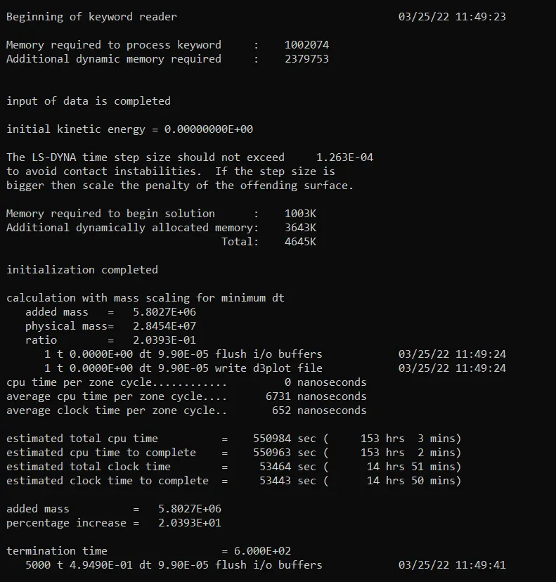
      2. The next control card is Control_Timestep card. As this analysis runs for a very large time period, in order to reduce the time taken for successful termination we have to assign tssfac and dt2ms. Whose multiple adds mass to elements and reduces the solving time. To check how this effects our solving time I've tried with different values of tssfac and dt2ms.
         1. 1st Iteration-
            • The values of tssfac and dt2ms are given below.
              
              • 
            • The solving time is given below
              • 
         2. 2nd Iteration-
            • The values of tssfac and dt2ms are given below.
              • 
            • The solving time is given below
              • 
         3. 3rd Iteration-
            • The values of tssfac and dt2ms are given below.
              • 
            • The solving time is given below
              • 
         4. 4th Iteration-
            • The values of tssfac and dt2ms are given below.
              • 
            • The solving time is given below
              • 
         5. 5th Iteration-
            • The values of tssfac and dt2ms are given below.
              • 
            • The solving time is given below
              • 
         6. 6th Iteration-
            • The values of tssfac and dt2ms are given below.
              • 
            • The solving time is given below
              • 
         7. 7th Iteration-
            • The values of tssfac and dt2ms are given below.
              • 
            • The solving time is given below
              • 
         8. 8th Iteration-
            • The values of tssfac and dt2ms are given below.
              • 
            • The solving time is given below
              • 
         9. 9th Iteration-
            • The values of tssfac and dt2ms are given below.
              • 
            • The solving time is given below
              • 
         10. 10th Iteration-
             • The values of tssfac and dt2ms are given below.
               • 
             • The solving time is given below
               • 
         11. 11th Iteration-
             • The values of tssfac and dt2ms are given below.
               • 
             • The solving time is given below
               • 
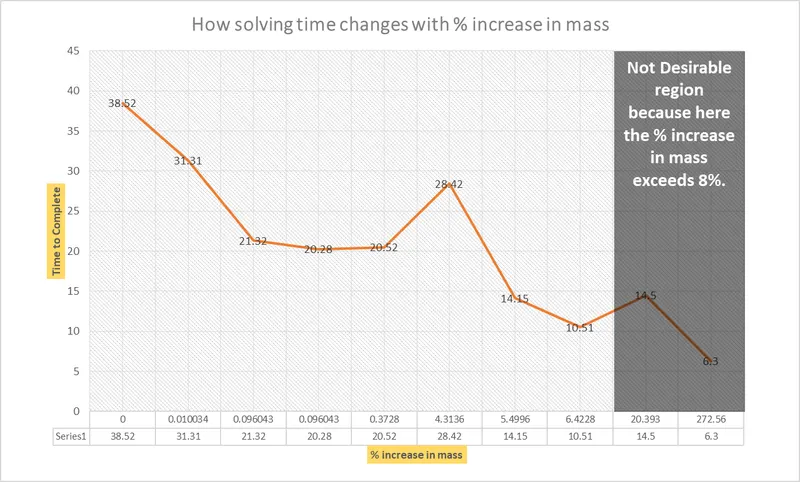
      3. The next step is to write down all the corresponding values of %increase in mass & solving time in an excel sheet. The data table is given below

         • %increase in mass	time to complete
           0	38.52
           0.010034	31.31
           0.096043	21.32
           0.096043	20.28
           0.3728	20.52
           4.3136	28.42
           5.4996	14.15
           6.4228	10.51
           20.393	14.5
           272.56	6.3

      4. The corresponding plots are shown below,
         • 
      5. From the above plot, we can conclude that in Explicit Analysis the least time it takes to solve the above situation is 10.51 hrs while respecting the 8% mass increase limit.
2. Implicit Analysis
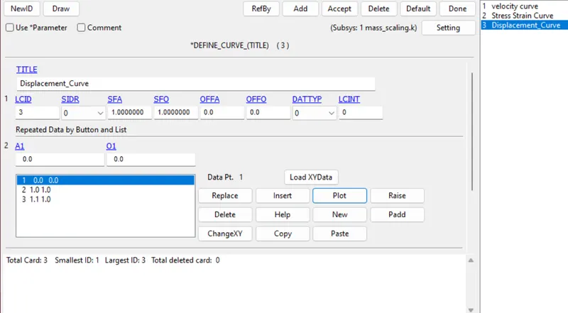
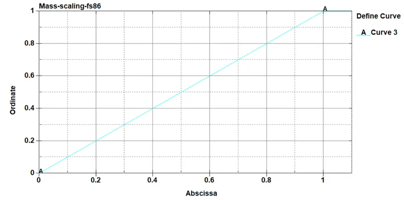
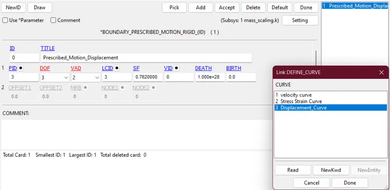
   1. The first step in implicit is to make the motion time-independent i.e. if the motion is velocity or acceleration in the case of explicit we've to makeshift the loading curve as such that the load changes to displacement type. By keeping this in mind I've changed the loading curve and motion type in the Boundary_Prescribed_Motion card.
      • The Define_Curve card is given below
        • 
        • 
      • The Boundary_Prescribed_Motion card is given below
        • 
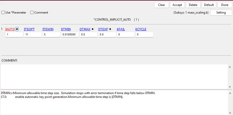
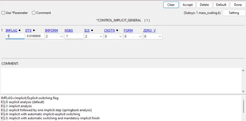
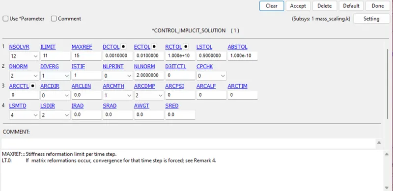
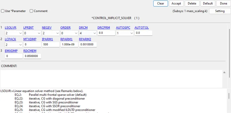
   2. The next step is to define Control cards, which change the analysis type from explicit to implicit. In the case of Implicit, we have to define multiple cards such as Implicit_Auto, Implicit_General, Implicit_Solution, Implicit_Solver & Termination cards.
      • In Implicit_Auto we have to define two main things one is the minimum time step and the other is the requirement of auto change of time step.
        • 
      • In Implicit_General we have to define the analysis type and the initial time step size.
        
        • 
      • For our case, we have to accept the default values of the Implicit_Solution card.
        • 
      • For our case, we have to accept the default values of the Implicit_Solver card
        • 
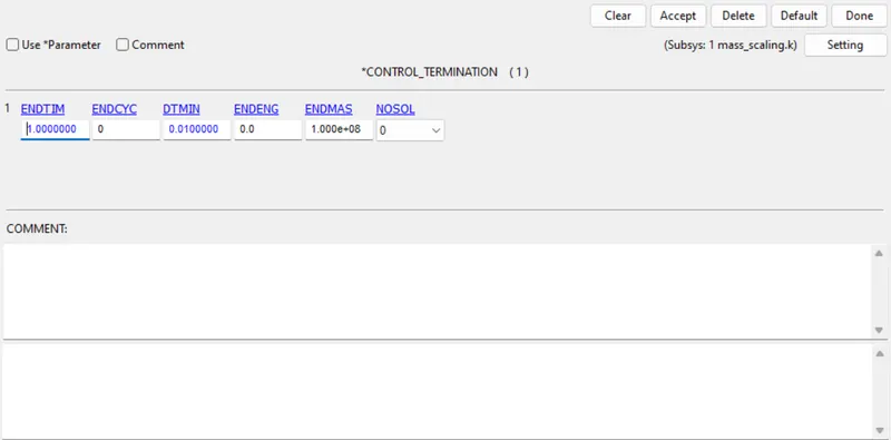
      • In the Termination card, we have to define the termination time of the analysis. As we are using implicit here no need to do mass scaling because the analysis we are doing is Quasi-Static type.
        
        • 
3. The next step is to define the database cards for post-processing.
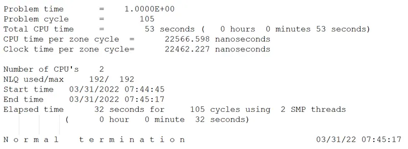
4. Let's open the message file and check the solving time for implicit. As we can see from below image the total elapsed time is 32 seconds.
   • 

• As we can see from above that the right knowledge of implicit and explicit can save us a lot of time in solving different types of problems.
• In this case, if we use explicit out of negligence we can end up wasting 15 hours. But the same problem just took 30 seconds to solve in implicit.
• The main takeaway from this challenge is that before starting the solution process in ls-dyna we have to decide that, by which solving method we try to solve the problem with proper reason.