Week 8: Literature review RANS derivation and analysis
Objective:
Apply Reynold's decomposition to the NS equations and come up with the expression for Reynold's stress.
- Explain understanding of the terms Reynold's stress
- What is turbulent viscosity? How is it different from molecular viscosity?
Theory:
What is Turbulence?
"Turbulence is an irregular motion which in general makes its appearance in fluids, gaseous or liquid when they flow past solid surfaces or even when neighboring streams of the same fluid flow past or over one another. "
Turbulence is the state of chaotic and unstable fluid flow, just opposite of Laminar flow. Y-Plus (Y+) is the non-dimensional distance of the first cell from the wall.
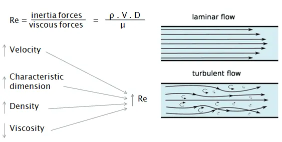
Turbulence is a continuous phenomenon that exists on a large range of length and time scales, which are still larger than molecular scales. In order to visualize turbulent flows, one often refers to turbulent eddies, which can be thought of as a local swirling motion whose characteristic dimension is on the order of the local turbulence length scale. Turbulent eddies also overlap in space, where larger eddies carry smaller ones. As there exists a large range of different scales (or turbulent eddy sizes), an energy cascade exists by which energy is transferred from the larger scales to the smaller scales, and eventually to the smallest scales where the energy is dissipated into heat by molecular viscosity.
Turbulence is commonly observed in everyday phenomena such as surf, fast-flowing rivers, billowing storm clouds, or smoke from a chimney, and most fluid flows occurring in nature or created in engineering applications are turbulent. Turbulence is caused by excessive kinetic energy in parts of a fluid flow, which overcomes the damping effect of the fluid's viscosity. For this reason, turbulence is commonly realized in low viscosity fluids. In general terms, in turbulent flow, unsteady vortices appear of many sizes which interact with each other, consequently drag due to friction effects increases. This increases the energy needed to pump fluid through a pipe. Turbulence can be exploited, for example, by devices such as aerodynamic spoilers on aircraft that "spoil" the laminar flow to increase drag and reduce lift.
Turbulence can be predicted by the dimensionless Reynolds number
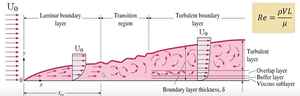
External Flow: Re<5e10^5 (Laminar Flow)
Re>5e10^5 (Turbulent Flow)
Internal Flow: Re<2300 (Laminar Flow)
Re>4000 (Turbulent Flow)
Navier Stokes Equations:
The movement of fluid in the physical domain is driven by various properties. For the purpose of bringing the behavior of fluid flow to light and developing a mathematical model, those properties have to be defined precisely to provide the transition between the physical and the numerical derivation. Velocity, pressure, temperature, density, and viscosity are the main properties that should be considered simultaneously when conducting the fluid flow examination. In accordance with the physical incidents such as combustion, multiphase flow, turbulence, mass transport, etc., those properties diversify enormously, which can be categorized into kinematic, transport, thermodynamic, and other properties.
It is relatively easy, for instance, to solve these equations for a flow between parallel plates or for the flow in a circular pipe. For more complex geometries, however, the equations need to be resolved depending upon the flow regime of interest, it is often possible to simplify these equations. In other cases, additional equations may be required. In the field of fluid dynamics, the different flow regimes are categorized using a non-dimensional number such as the Reynolds number and the Mach number.
All the governing equations are based on the laws of conservation. The Navier- Stokes equations are applied to a mathematical model to examine changes in those properties during dynamic or thermal interactions. The equations are adjustable regarding the content of the problem and are expressed based on the principles of conservation of mass, momentum, and energy.
Note: All the equations are in a 2D cartesian coordinate system
Governing Equations for incompressible flow:
Continuity Equation - Conservation of Mass:
`(delu)/(delx)+(delv)/(dely)=0`
Momentum Equation
`rho[(delu)/(delt)+u(delu)/(delx) +v(delu)/(dely)]=-(delp)/(delx)+mu (del^2u)/(dely^2)`
Energy Equation
`rhounderset(c)() [(delT)/(delt) +u(delT)/(delx) + v(delT)/(dely)] = K[(del^2T)/(delx^2) + (del^2T)/(dely^2)] + mu ((delu)/(dely))^2`
Reynolds-averaged Navier Stokes Equations (RANS):
Although statistical theory and numerical simulation (DNS) are viable options, most of the research on turbulent flow analysis in the past century has used the concept of time averaging. Applying the time averaging to the basic equations of motion yields the Reynolds equations, which involve both mean and fluctuating quantities. One then attempts to model the fluctuation terms by relating them to mean properties or their gradients. This approach may now be yielding diminishing returns. Lumley (1989) gives a stimulating discussion of how time averaging might outlive its usefulness. The Reynolds equations are far from obsolete, however, and form the basis of most engineering analyses of turbulent flow.
Need of RANS:
Most of the engineering simulations need to be computationally effective (with less computational effort). To capture the minute effects of turbulence DNS can not be applied effectively (high computation effort required) and it requires the mesh size to be of order (1e-9 or less) to be in compliance with CFL number and small-time steps, it is going to be computationally inviable. Hence, to be computationally viable, engineers depend upon the time-averaged solutions, where the turbulence of engineering needs is captured effectively. Here the time step used is large compared to the relevant period of fluctuations of components. Hence a coarse grid than the one used for DNS can be used which will reduce the computational effort.
Reynold's Decomposition:
In this process, we decompose a function into a mean and fluctuating function.
`u(x, y, z, t) = baru(x,y,z) + uprime(x, y, z, t)`
`v(x, y, z, t) = barv(x,y,z) + vprime(x, y, z, t)`
`w(x, y, z, t) = ubrace(barw(x,y,z))_("averaged Velocity") + ubrace(wprime(x, y, z, t))_("Velocity Fluctuation")`
The mean time average velocity is a function of space while the fluctuating velocity is the function of space and time both.
Now, On integrating Average velocity from 0 to `tunderset("int")`,
`baru(x, y) =(1)/(tunderset("int")())int_0^(tunderset("int")( )) u(x,y, t)dt`
`barv(x, y) =(1)/(tunderset("int")())int_0^(tunderset("int")( )) v(x,y,t)dt`
Since `baru`is the averaging operator
`baru = (1)/(tunderset("int")())int_0^(tunderset("int")())(baru + uprime)dt`
`baru = (1)/(tunderset("int")())int_0^(tunderset("int")())(baru)dt+(1)/(tunderset("int")())int_0^(tunderset("int")())(uprime)dt`
As we know, `baru`is not a function of time,
`baru = baru [[tunderset("int")()-0]/[tunderset("int")()]]+(1)/(tunderset("int")())int_0^(tunderset("int")())(uprime)dt`
`cancel(baru) = cancel(baru) +(1)/(tunderset("int")())int_0^(tunderset("int")())(uprime)dt`
Therefore,
`(1)/(tunderset("int")())int_0^(tunderset("int")())(uprime)dt = 0`
Let's substitute this decomposition into the continuity equation,
`(delu)/(delx) + (delv)/(dely) =0`
`(del)/(delx)(baru +uprime) + (del)/(dely)(barv +vprime) = 0`
Taking time average of the above equation,
`(1)/(tunderset("int")())int_0^(tunderset("int")())(del)/(delx)(baru +uprime)dt + (1)/(tunderset("int")())int_0^(tunderset("int")())(del)/(dely)(barv +vprime)dt = 0`
`(1)/(tunderset("int")())int_0^(tunderset("int")())(del)/(delx)barudt +(1)/(tunderset("int")())int_0^(tunderset("int")())(del)/(delx)uprimedt + (1)/(tunderset("int")())int_0^(tunderset("int")())(del)/(dely)barvdt +(1)/(tunderset("int")())int_0^(tunderset("int")())(del)/(dely)vprimedt = 0`
As derived earlier, average velocity fluctuation is equal to zero,
`(1)/(tunderset("int")())int_0^(tunderset("int")())(del)/(delx)barudt +cancel((1)/(tunderset("int")())int_0^(tunderset("int")())(del)/(delx)uprimedt) + (1)/(tunderset("int")())int_0^(tunderset("int")())(del)/(dely)barvdt +cancel((1)/(tunderset("int")())int_0^(tunderset("int")())(del)/(dely)vprimedt) = 0`
`(1)/(tunderset("int")())int_0^(tunderset("int")())(del)/(delx)barudt + (1)/(tunderset("int")())int_0^(tunderset("int")())(del)/(dely)barvdt = 0`
By solving the Definite Integral,
`(delbaru)/(delx) [[tunderset("int")()-0]/[tunderset("int")()]]+ (delbarv)/(dely) [[tunderset("int")()-0]/[tunderset("int")()]]= 0`
`(delbaru)/(delx)+ (delbarv)/(dely)= 0`
This implies the Time-averaged equation satisfies the continuity equation.
Let's apply Reynold's Decomposition on Momentum Equation,
`rho[(delu)/(delt)+u(delu)/(delx) +v(delu)/(dely)]=-(delp)/(delx)+mu (del^2u)/(dely^2)`
Dividing both side by `rho`,we get,
`(delu)/(delt)+u(delu)/(delx) +v(delu)/(dely)=(-1)/(rho)(delp)/(delx)+(mu)/rho(del^2u)/(dely^2)`
Replacing `mu/rho = gamma` by kinematic viscocity,
`(delu)/(delt)+u(delu)/(delx) +v(delu)/(dely)=(-1)/(rho)(delp)/(delx)+gamma.(del^2u)/(dely^2)`
As we know, from the continuity equation,
`(delu)/(delx)+(delv)/(dely)=0`
Multiplying `u`on both sides,
`u.((delu)/(delx)+(delv)/(dely))=0`
Adding modified continuity equation term on left side,
`[(delu)/(delt)+u.(delu)/(delx) +v.(delu)/(dely)] + u.[(delu)/(delx)+(delv)/(dely)] =(-1)/(rho).(delp)/(delx)+gamma.(del^2u)/(dely^2)`
On simplifying we get,
`[(delu)/(delt)+2u.(delu)/(delx) +v.(delu)/(dely) + u.(delv)/(dely)] =(-1)/(rho).(delp)/(delx)+gamma.(del^2u)/(dely^2)`
As per derivative product rule,
`(del(u.v))/(dely) = v.(delu)/(dely) + u.(delv)/(dely)`
Using this rule in following equation,
`[(delu)/(delt)+2u.(delu)/(delx) +ubrace(color(red)(v.(delu)/(dely) + u.(delv)/(dely))] =(-1)/(rho).(delp)/(delx)+gamma.(del^2u)/(dely^2)`
`[(delu)/(delt)+2u.(delu)/(delx) +color(blue)((del(u.v))/(dely)] =(-1)/(rho).(delp)/(delx)+gamma.(del^2u)/(dely^2)`
Using square rule in derivative,
`[(delu)/(delt)+(del(u^2))/(delx) +(del(u.v))/(dely)] =(-1)/(rho).(delp)/(delx)+gamma.(del^2u)/(dely^2)`
Now, lets substitute
`u = baru + uprime`
`v = barv + vprime`
Equation becomes,
`(del(baru + uprime))/(delt)+(del(baru + uprime)^2)/(delx) +(del(baru + uprime).(barv + vprime))/(dely) =(-1)/(rho).(del(barp + pprime))/(delx)+gamma.(del^2(baru + uprime))/(dely^2)`
`(delbaru)/(delt) + (deluprime)/(delt)+(delbaru^2)/(delx) +(deluprime^2)/(delx) + (del (2.baru.uprime))/(delx) +(del(baru.barv))/(dely) +(del(baru.vprime))/(dely) +(del(uprime.barv))/(dely) +(del(uprime.vprime))/(dely)=-(1)/(rho).(delbarp)/(delx)-(1)/(rho).(delpprime)/(delx)+gamma.(del^2baru)/(dely^2) +gamma.(del^2uprime)/(dely^2)`
As derived earlier, Velocity fluctuation derivatives would result into zero when definite reynold's decomposition is applied,
`int_0^(tunderset("int")())[(delbaru)/(delt)dt + (deluprime)/(delt)dt+(delbaru^2)/(delx) dt+(deluprime^2)/(delx) dt+ (del (2.baru.uprime))/(delx)dt +(del(baru.barv))/(dely) dt +(del(baru.vprime))/(dely) dt +(del(uprime.barv))/(dely) dt +(del(uprime.vprime))/(dely) dt ]=int_0^(tunderset("int")())[-(1)/(rho).(delbarp)/(delx) dt -(1)/(rho).(delpprime)/(delx) dt +gamma.(del^2baru)/(dely^2) dt +gamma.(del^2uprime)/(dely^2) dt]`
`int_0^(tunderset("int")())[(delbaru)/(delt) dt + (deluprime)/(delt) dt +(delbaru^2)/(delx) dt +(deluprime^2)/(delx) dt + (del (2.baru.uprime))/(delx) dt +(del(baru.barv))/(dely) dt +(del(baru.vprime))/(dely) dt +(del(uprime.barv))/(dely) dt +(del(uprime.vprime))/(dely) dt ]=int_0^(tunderset("int")())[-(1)/(rho).(delbarp)/(delx) dt -(1)/(rho).(delpprime)/(delx) dt +gamma.(del^2baru)/(dely^2) dt +gamma.(del^2uprime)/(dely^2) dt ]`
`int_0^(tunderset("int")())[(delbaru)/(delt) dt + cancel((deluprime)/(delt) dt) +(delbaru^2)/(delx) dt +(deluprime^2)/(delx) dt +cancel((del (2.baru.uprime))/(delx) dt )+(del(baru.barv))/(dely) dt +cancel((del(baru.vprime))/(dely) dt )+cancel((del(uprime.barv))/(dely) dt )+(del(uprime.vprime))/(dely) dt ]=int_0^(tunderset("int")())[-(1)/(rho).(delbarp)/(delx) dt -cancel((1)/(rho).(delpprime)/(delx) dt) +gamma.(del^2baru)/(dely^2) dt +cancel(gamma.(del^2uprime)/(dely^2) dt) ]`
After rearranging this equation, we will get,
`(delbaru)/(delt)+(delbaru^2)/(delx)+(deluprime^2)/(delx) +(del(baru.barv))/(dely) + (del(uprime.vprime))/(dely) = -(1)/(rho).(delbarp)/(delx) +gamma.(del^2baru)/(dely^2)`
`(delbaru)/(delt)+(delbaru^2)/(delx) +(del(baru.barv))/(dely) = -(1)/(rho).(delbarp)/(delx) +gamma.(del^2baru)/(dely^2) - 1/(tunderset("int")())int_0^(tunderset("int")())(deluprime^2)/(delx) dt - 1/(tunderset("int")())int_0^(tunderset("int")())(del(uprime.vprime))/(dely) dt`
`(delbaru)/(delt)+(delbaru^2)/(delx) +(del(baru.barv))/(dely) = -(1)/(rho).(delbarp)/(delx) + gamma.(del^2baru)/(dely^2) - 1/(tunderset("int")())int_0^(tunderset("int")())(del(uprime.vprime))/(dely) dt ubrace(- 1/(tunderset("int")())int_0^(tunderset("int")())(deluprime^2)/(delx) dt)_("negelecting this term")`
After neglecting `uprime^2`, we get,
`(delbaru)/(delt)+(delbaru^2)/(delx) +(del(baru.barv))/(dely) = -(1)/(rho).(delbarp)/(delx) + gamma.(del^2baru)/(dely^2) - 1/(tunderset("int")())int_0^(tunderset("int")())(del(uprime.vprime))/(dely) dt`
`((delbaru)/(delt)+(delbaru^2)/(delx) +(del(baru.barv))/(dely)) = -(1)/(rho).(delbarp)/(delx) +gamma.(del^2baru)/(dely^2) - 1/(tunderset("int")())int_0^(tunderset("int")())(del(uprime.vprime))/(dely) dt`
`((delbaru)/(delt)+(delbaru^2)/(delx) +(del(baru.barv))/(dely)) = -(1)/(rho).(delbarp)/(delx) +gamma.(del^2baru)/(dely^2) - 1/(tunderset("int")())int_0^(tunderset("int")())(del(uprime.vprime))/(dely) dt`
`((delbaru)/(delt)+(delbaru^2)/(delx) +(del(baru.barv))/(dely)) = -(1)/(rho).(delbarp)/(delx) +(1)/(rho).(del)/(delx)(mu.(delbaru)/(dely)-rho.uprime.vprime)`
Unsteady Reynold's Average Navier Stokes equation:
`rho.((delbaru)/(delt)+(delbaru^2)/(delx) +(del(baru.barv))/(dely)) = -(delbarp)/(delx) +(del)/(delx)(mu.(delbaru)/(dely)-ubrace(rho.uprime.vprime)_("Reynolds Stress"))`
The above equation `rho.uprime.vprime`represents added stress on the fluid.
Reynolds Stress :
Reynolds stress is the component of the total stress tensor in a fluid obtained from the averaging operation over the Navier-Stokes equations to account for turbulent fluctuations in fluid momentum.
`tauprimeunderset(uv) () = -rho. uprime.vprime`
What is Turbulent Viscosity? How is it different from Molecular Viscosity?
The turbulent viscosity is also called eddy viscosity. In the study of turbulence in fluids, a common practical strategy is to ignore the small-scale vortices (or eddies) in the motion and to calculate a large-scale motion with an effective viscosity, called the "eddy viscosity", which characterizes the transport and dissipation of energy in the smaller-scale flow (see large eddy simulation). In contrast to the viscosity of the fluid itself, which must be positive by the second law of thermodynamics, the eddy viscosity can be negative.
Molecular viscosity is the same as viscosity. The Coefficient of Molecular Viscosity is the same value as dynamic viscosity. Molecular viscosity is the transport of mass motion momentum solely by the random motions of individual molecules not moving together in coherent groups. Molecular viscosity is analogous in laminar ow to eddy viscosity in a turbulent flow.
The dynamic viscosity or molecular viscosity is a macroscopic fluid property, you can think of it as what distinguishes honey and water. And the eddy viscosity or turbulent viscosity is a flow property emerging from the increased momentum transport through the flow field due to turbulent velocity fluctuations.