Week 5: Prandtl Meyer Shock problem

Shock Flow Boundary Conditions:

Boundary conditions, which exist in the form of mathematical equations, exert a set of additional constraints to the problem on specified boundaries. The concept of boundary conditions applies to both ordinary and partial differential equations. There are five types of boundary conditions: Dirichlet, Neumann, Robin, Mixed, and Cauchy, within which Dirichlet and Neumann are predominant.

To understand the difference, let us take a look at an ordinary differential equation du/dx + u=0 in the domain[a,b]

Dirichlet Condition:

In the Dirichlet boundary condition, the value of the function is specified at the boundary. This boundary condition is generally used while solving linear problems.

We have the Dirichlet boundary condition when the boundary prescribes a value to the dependent variable(s). A Dirichlet boundary condition for the above ODE looks like

y(a)=A

y(b)=B

For example, in a 1D heat transfer problem, when both ends of a wire are maintained in a water bath with constant temperatures, the above boundary condition will be appropriate.

Neumann Condition:

In the Neumann boundary condition, the value of the normal derivative of a function is specified. It is imposed on an ordinary or a partial differential equation and specifies the values that the derivative of a solution is assigned to the boundary of the domain. This boundary condition is generally used in non-linear
problems.

In the Neumann boundary condition, the derivative of the dependent variable is known in all parts of the boundary:

y′(a)=α

y′(b)=β

In the above heat transfer example, if heaters exist at both ends of the wire, via which energy would be added at a constant rate, the Neumann boundary condition will apply.

Robin Condition:

It is the combination of both the above boundary conditions, specified at both ends.

The Robin boundary condition is a weighted combination of the Dirichlet boundary and the Neumann boundary condition in all the parts of the boundary:χ1⋅y(a)+χ2⋅y′(a)=Aαχ1⋅y(b)+χ2⋅y′(b)=Bβ

where Xi's are constants representing the weights. The Dirichlet, Neumann, and Robin are also called the first-type, second-type, and third-type boundary conditions, respectively.

Mixed Condition:

On one end there is a Dirichlet boundary condition and on the other end, there is a Robin boundary condition. The mixed boundary condition refers to the cases in
which Dirichlet boundary conditions are assigned in one end of the boundary while Neumann boundary conditions are assigned to the other end.

Accordingly, for the above ODE, the following is a typically mixed boundary condition:

y(a)=A

y′(b)=β

Cauchy Condition:

While being less common, Cauchy boundary conditions are also used in second-order differential equations, in which one may specify the value of the function y and the value of the derivative y at a given point:

u(a)=A

u′(a)=α

Therefore, the Cauchy boundary conditions correspond to imposing a Dirichlet and a Neumann boundary conditions simultaneously.

Boundary Condition for Shock flow problems

The values of the variables like temperature, Mach no., velocity, pressure are not available at the initiation of the problem. At a supersonic outlet boundary condition, nothing is specified and all listed variables are extrapolated from the interior domain.

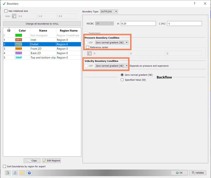
Only the Normal derivative (Normal with respect to the outlet boundary) of variables are specified as 0 (or Zero Gradient). However, if any pressure value or velocity is specified at the outlet the solution will not converge and become unstable.

In the Neumann boundary condition, the value of the gradient of the dependent variable is provided along the boundary of the domain.

In supersonic flow, characterized by abrupt changes in state parameters, a
steady value of parameters. Hence extrapolated Neumann boundary conditions are employed for shock waves and supersonic conditions.

What are Shock Waves?

In physics, a shock wave (also spelled shockwave), or shock, is a type of propagating disturbance that moves faster than the local speed of sound in the medium. Like an ordinary wave, a shock wave carries energy and can propagate through a medium but is characterized by an abrupt, nearly discontinuous, change in pressure, temperature, and density of the medium.

For the purpose of comparison, in supersonic flows, additional increased expansion may be achieved through an expansion fan, also known as a Prandtl–Meyer expansion fan. The accompanying expansion wave may approach and eventually collide and recombine with the shock wave, creating a process of destructive interference. The sonic boom associated with the passage of a supersonic aircraft is a type of sound wave produced by constructive interference.

The energy and speed of a shock wave alone dissipate relatively quickly with distance. When a shock wave passes through matter, energy is preserved but entropy increases. This change in the matter's properties manifests itself as a decrease in the energy which can be extracted as work, and as a drag force on supersonic objects; shock waves are strongly irreversible processes.

Shock waves can be:

Normal:

At 90° (perpendicular) to the shock medium's flow direction.

In elementary fluid mechanics utilizing ideal gases, a shock wave is treated as a discontinuity where entropy increases over a nearly infinitesimal region. Since no fluid flow is discontinuous, a control volume is established around the shock wave, with the control surfaces that bound this volume parallel to the shock wave (with one surface on the pre-shock side of the fluid medium and one on the post-shock side). The two surfaces are separated by a very small depth such that the shock itself is entirely contained between them. At such control surfaces, momentum, mass flux, and energy are constant; within combustion, detonations can be modeled as heat introduction across a shock wave. It is assumed the system is adiabatic (no heat exits or enters the system) and no work is being done. The Rankine–Hugoniot conditions arise from these considerations.

Taking into account the established assumptions, in a system where the downstream properties are becoming subsonic: the upstream and downstream flow properties of the fluid are considered isentropic. Since the total amount of energy within the system is constant, the stagnation enthalpy remains constant over both regions. Though, entropy is increasing; this must be accounted for by a drop in stagnation pressure of the downstream fluid.

Oblique:

At an angle to the direction of flow.

When analyzing shock waves in a flow field, which are still attached to the body, the shock wave which is deviating at some arbitrary angle from the flow direction is termed oblique shock. These shocks require a component vector analysis of the flow; doing so allows for the treatment of the flow in an orthogonal direction to the oblique shock as a normal shock.

Bow:

Occurs upstream of the front (bow) of a blunt object when the upstream flow velocity exceeds Mach 1.

When an oblique shock is likely to form at an angle that cannot remain on the surface, a nonlinear phenomenon arises where the shock wave will form a continuous pattern around the body. These are termed bow shocks. In these cases, the 1d flow model is not valid and further analysis is needed to predict the pressure forces which are exerted on the surface.

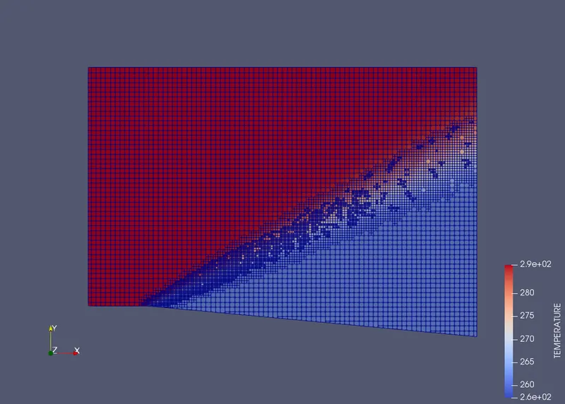
Aim: In the Prandtl Meyer shock problem, predict the effects of SGS temperature value on cell count and the shock location.

Introduction and Theory:

A supersonic expansion fan, technically known as Prandtl–Meyer expansion fan, a two-dimensional simple wave, is a centered expansion process that occurs when a supersonic flow turns around a convex corner. The fan consists of an infinite number of Mach waves, diverging from a sharp corner. When a flow turns around a smooth and circular corner, these waves can be extended backward to meet at a point.

Each wave in the expansion fan turns the flow gradually (in small steps). It is physically impossible for the flow to turn through a single "shock" wave because this would violate the second law of thermodynamics.^[1]

Across the expansion fan, the flow accelerates (velocity increases) and the Mach number increases, while the static pressure, temperature, and density decrease. Since the process is isentropic, the stagnation properties (e.g. the total pressure and total temperature) remain constant across the fan.

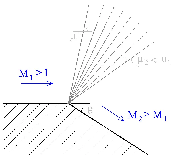
1. As Suggested, Channel flow simulation has been set up in CONVERGE.
2. In this shock wave simulation, Air is flowing through the given geometry from one to another end. This Geometry has a divergent angle which is causing the shock wave.
3. Having this difference in pressure makes air flow from a high-pressure point to a low-pressure point. Sudden change is geometry and deviation in variables like density and temperature of molecules causing the shock wave.
5. During this simulation, the temperature is considered as 286K

Case Setup:

1. In converge, we are selecting a Time-based application for this project.
2. For materials, we are selecting a predefined mixture as Air which has Oxygen and nitrogen as species of this mixture.
3. In this project, turbulence models are not included since there is no Reynolds stress because the flow is inviscid. This project was running for the maximum limit of 25000 cycles and after every 100 cycles restart files and result snapshot was recorded.
4. The solver parameters were defaulted to Navier stokes equation-based PISO solver.
5. This particular project is an example of steady-state simulation.
6. The channel is assigned different boundary conditions:
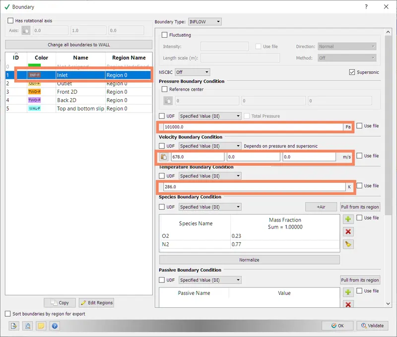
- inlet conditions at specified value Dirichlet Condition(High pressure point)

- Static Pressure = 101000 Pa

- Velocity = 678 m/s

- Temperature = 286 K

- the outlet at Zero Neumann Condition like pressure, velocity and temperature (low-pressure point)
- Slip Wall Condition - because of supersonic inviscid flow(top and bottom)
- 2D sliced walls (front and back)

The 2D planar assumption is used because the flow gradients along the z-direction are negligible when compared to the other two directions. By reducing the model to 2D, the Prandtl Meyer can be simulated and analyzed cost-effectively compared to a full 3D model.

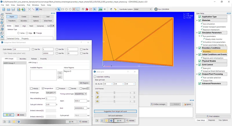
7. After setting up the grid size(0.8m), variables for post-processing were selected. (velocity, mass flow, pressure, density, temperature). In this problem, we are doing temperature-based Adaptive mesh refinement. This is based on the second derivative of Temperature.
8. After exporting input files, using CYGWIN (command prompt) was used to simulate the project setup.
9. Output files were later converted using CONVERGE studio for post-processing in ParaView.

Animation:

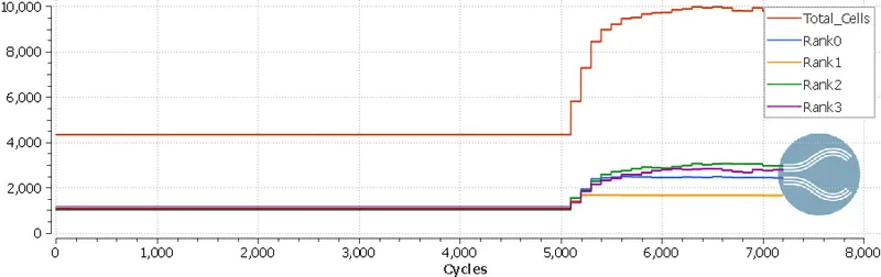
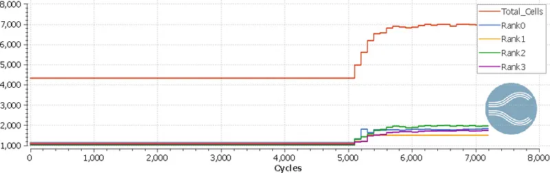
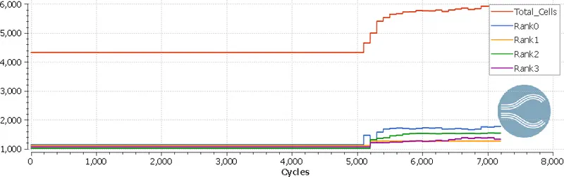
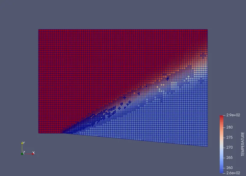
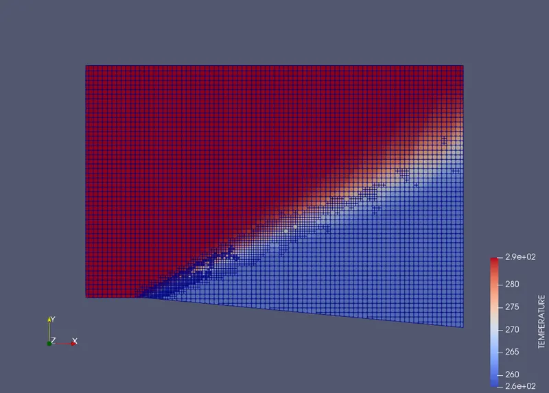
Results with different SGS values for Adaptive mesh refinement:

SGS = 0.03 K	SGS = 0.05 K	SGS = 0.07 K
Cell count = 10000 (max)	Cell Count = 7000 (max)	Cell count = 6000 (max)

Summary of Comparative results:
1. Total cell counts decrease as adaptive mesh refinement Temp SGS increases from 0.03 K to 0.07. This is because temperature derivative tolerance is higher, it can accommodate more base grid size mesh.
2. So if you want to refine the mesh size to lower the value of the temperature SGS criterion, you can get more refined results but it will increase computation cost. But it will definitely increase accuracy.

3. Analogically, this is like having more pixels in an image. With finer pixels or more number pixels will improve the quality of image. In this case, this is actually increasing solution accuracy.

Conclusion:

In the Prandtl Meyer shock problem, the effects of SGS temperature value on cell count and the shock location have been explored.