Week 4.1: Project Steady state simulation of flow over a throttle body
Aim: Perform a Steady-state flow simulation over a throttle body inside the elbow manifold.
Introduction and Theory:
1. As Suggested, Steady-state flow simulation over throttle body has been set up in CONVERGE.
2. In this flow simulation, Air is flowing through the elbow from one to another end.
3. This elbow has a throttle plate. One end is maintained at just 1.5 bar and another at 1 bar.
4. Having this difference in pressure makes airflow from a high-pressure point to a low-pressure point.
Steady-state flow refers to the condition where all the flow parameters do not change over time throughout the entire domain. Otherwise, it is called transient (unsteady) flow. A steady-state flow simulation can generally save a lot of computer resources and CPU time.
Case Setup:
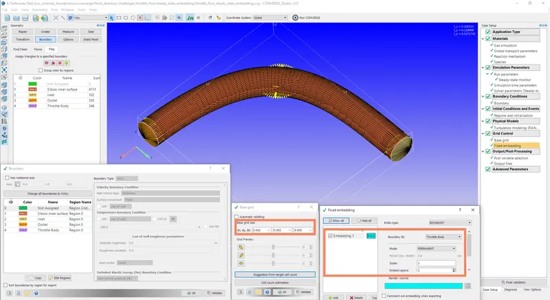
1. In converge, we are selecting a Time-based application for this project.
2. For materials, we are selecting a predefined mixture as Air which has Oxygen and nitrogen as species of this mixture.
3. In this project, the turbulence model used is RNE k-epsilon. This project was running for the maximum limit of 15000 cycles and after every 100 cycles restart files and result snapshot was recorded.
4. The solver parameters were defaulted to Navier stokes equation-based PISO solver.
5. This particular project is an example of steady-state simulation.
6. The elbow and throttle body are assigned with different boundary conditions:
i. inlet (High-pressure point)
ii. outlet (low-pressure point)
iii. Elbow Walls (Fixed wall)
iv. Throttle Body (Fixed wall condition for steady-state simulation)
7. After setting up the grid size, fixed embedding parameters; variables for post-processing were selected. (velocity, mass flow, pressure, density, temperature)
8. After exporting input files, using CYGWIN (command prompt) was used to simulate the project setup.
9. Output files were later converted using CONVERGE studio for post-processing in ParaView.
10. Maximum CFL limit is set at 1.00
11. base grid size is 0.002 m.
12. The bounding box dimensions are as following:
Ix= 0.106314 m
Iy= 0.119998 m
Iz= 0.0171742 m
Summary of Results:
Here are the results of this simulation,
| Pressure Contour | 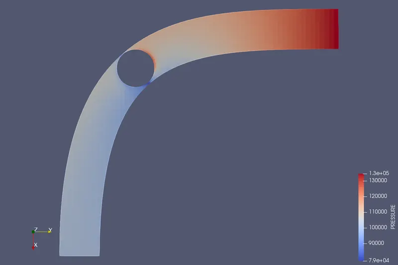 |
| Velocity Contour | 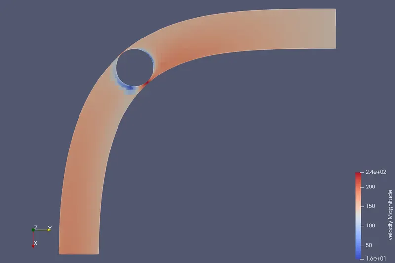 |
| Flow direction Glyph | 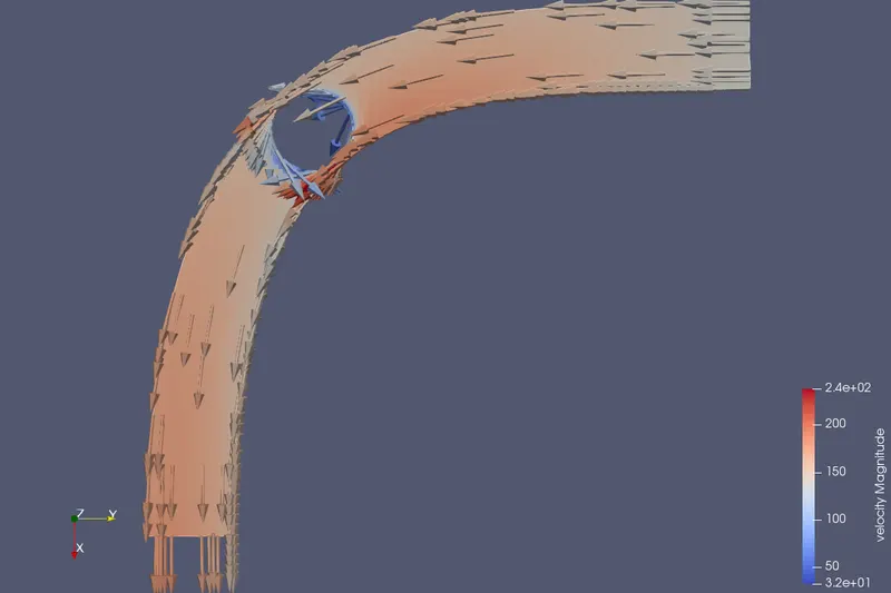 |
|
Mesh |
 |
| Outlet Pressure Plot | 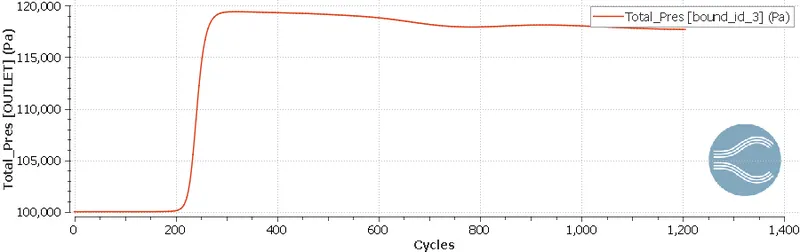 |
| Velocity Plot | 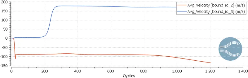 |
| Inlet Mass Flow Rate | 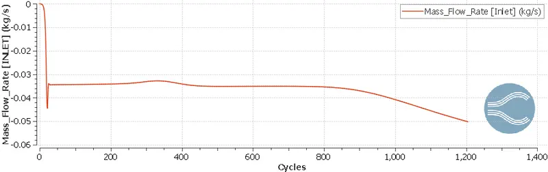 |
| Outlet Mass Flow Rate | 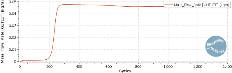 |
| Total Cell Count | 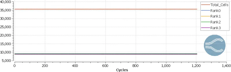 |
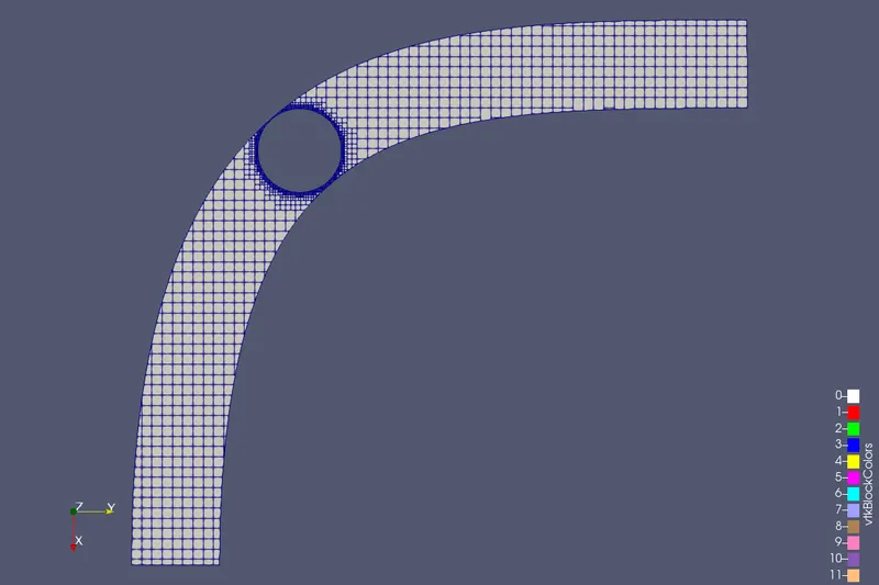
1. Total cell counts (no. of elements) in this simulation were about 36000 as the base grid size was about 0.002m. Also, for a better understanding of flow patterns over the throttle body, we added local refinement. In other terms, we added embedding to just near the throttle body.
2. Near the throttle body, when air is hitting the body, pressure is increasing due to flow resistance. And as air is leaving the trailing part of the throttle body, pressure is decreasing.
Animation:
Conclusion:
Steady-state flow simulation with fixed embedding mesh configurations has been analyzed and plots, contours have been obtained using ParaView.